Process-Map Style Outputs (Directly Follows Graphs - DFGs)

Packages like bupaR (for R) and pm4py (for Python) are designed for process mining on real-world process data.

However, there are a lot of useful visualisations that we can borrow from the process mining world and adapt for simulation, aiding in communicating processes with non-technical stakeholders, as well as verifying and debugging our model at various levels of granularity.

What do we mean by a process map? Well, it could be an output like this:

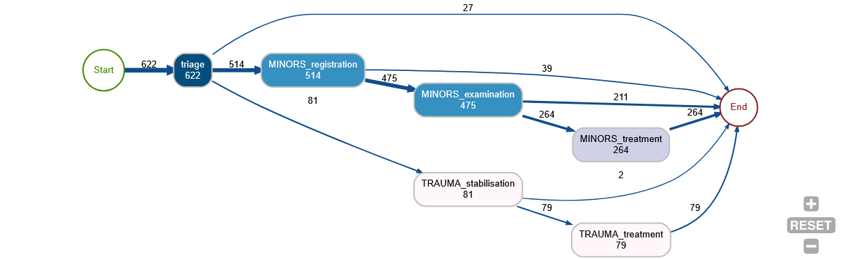
This gives us a quick overview of

• the number of entities that reach each stage (the numbers in the ‘nodes’ - the boxes)
• the number of people moving between each stage (the numbers on the ‘edges’ - the links)
• all of the possible pathways observed through the system
• the relative likeliness of each branch at each point (the thickness of the lines between the ‘edges’)

Vidigi allows for the creation of these types of outputs in three different ways: - static outputs using the Graphviz library - interactive outputs in jupyter notebooks using ipycytoscape - interactive outputs in streamlit web apps using streamlit-cytoscape

In this section, we’ll explore each of these.

We’ll start with a set of standard imports.

import pandas as pd

Example 1 - A simple linear pathway

from examples.feat_process_maps.logger_model import Trial, g

NoteView Imported Code, which has had logging steps added at the appropriate points in the ‘model’ class

import simpy
import numpy as np
import pandas as pd
from vidigi.logging import EventLogger
from vidigi.resources import VidigiStore
from sim_tools.distributions import Lognormal, Exponential
import random


# Class to store global parameter values.  We don't create an instance of this
# class - we just refer to the class blueprint itself to access the numbers
# inside.
class g:
    """
    Create a scenario to parameterise the simulation model

    Parameters:
    -----------
    random_number_set: int, optional (default=DEFAULT_RNG_SET)
        Set to control the initial seeds of each stream of pseudo
        random numbers used in the model.

    n_cubicles: int
        The number of treatment cubicles

    trauma_treat_mean: float
        Mean of the trauma cubicle treatment distribution (Lognormal)

    trauma_treat_var: float
        Variance of the trauma cubicle treatment distribution (Lognormal)

    arrival_rate: float
        Set the mean of the exponential distribution that is used to sample the
        inter-arrival time of patients

    sim_duration: int
        The number of time units the simulation will run for

    number_of_runs: int
        The number of times the simulation will be run with different random number streams

    """

    random_number_set = 42

    n_cubicles = 4
    trauma_treat_mean = 40
    trauma_treat_var = 5

    arrival_rate = 5

    sim_duration = 600
    number_of_runs = 100


# | code-fold: true
# | code-summary: "Show the patient class code"
class Patient:
    """
    Class defining details for a patient entity
    """

    def __init__(self, p_id):
        """
        Constructor method

        Params:
        -----
        identifier: int
            a numeric identifier for the patient.
        """
        self.id = p_id
        self.arrival = -np.inf
        self.wait_treat = -np.inf
        self.total_time = -np.inf
        self.treat_duration = -np.inf


# Class representing our model of the clinic.
class Model:
    """
    Simulates the simplest minor treatment process for a patient

    1. Arrive
    2. Examined/treated by nurse when one available
    3. Discharged
    """

    # Constructor to set up the model for a run.  We pass in a run number when
    # we create a new model.
    def __init__(self, run_number):
        # Create a SimPy environment in which everything will live
        self.env = simpy.Environment()

        # Store the passed in run number
        self.run_number = run_number

        # By passing in the env we've created, the logger will default to the simulation
        # time when populating the time column of our event logs
        self.logger = EventLogger(env=self.env, run_number=self.run_number)

        # Create a patient counter (which we'll use as a patient ID)
        self.patient_counter = 0

        # Create an empty list to hold our patients
        self.patients = []

        # Create our distributions
        self.init_distributions()

        # Create our resources
        self.init_resources()

    def init_distributions(self):
        self.patient_inter_arrival_dist = Exponential(
            mean=g.arrival_rate, random_seed=self.run_number * g.random_number_set
        )

        self.treat_dist = Lognormal(
            mean=g.trauma_treat_mean,
            stdev=g.trauma_treat_var,
            random_seed=self.run_number * g.random_number_set,
        )

    def init_resources(self):
        """
        Init the number of resources

        Resource list:
            1. Nurses/treatment bays (same thing in this model)

        """
        self.treatment_cubicles = VidigiStore(self.env, num_resources=g.n_cubicles)

    # A generator function that represents the DES generator for patient
    # arrivals
    def generator_patient_arrivals(self):
        # We use an infinite loop here to keep doing this indefinitely whilst
        # the simulation runs
        while True:
            # Increment the patient counter by 1 (this means our first patient
            # will have an ID of 1)
            self.patient_counter += 1

            # Create a new patient - an instance of the Patient Class we
            # defined above.  Remember, we pass in the ID when creating a
            # patient - so here we pass the patient counter to use as the ID.
            p = Patient(self.patient_counter)

            # Store patient in list for later easy access
            self.patients.append(p)

            # Tell SimPy to start up the attend_clinic generator function with
            # this patient (the generator function that will model the
            # patient's journey through the system)
            self.env.process(self.attend_clinic(p))

            # Randomly sample the time to the next patient arriving.  Here, we
            # sample from an exponential distribution (common for inter-arrival
            # times), and pass in a lambda value of 1 / mean.  The mean
            # inter-arrival time is stored in the g class.
            sampled_inter = self.patient_inter_arrival_dist.sample()

            # Freeze this instance of this function in place until the
            # inter-arrival time we sampled above has elapsed.  Note - time in
            # SimPy progresses in "Time Units", which can represent anything
            # you like (just make sure you're consistent within the model)
            yield self.env.timeout(sampled_inter)

    # A generator function that represents the pathway for a patient going
    # through the clinic.
    # The patient object is passed in to the generator function so we can
    # extract information from / record information to it
    def attend_clinic(self, patient):
        self.logger.log_arrival(entity_id=patient.id)

        self.arrival = self.env.now

        self.logger.log_queue(entity_id=patient.id, event="treatment_wait_begins")

        with self.treatment_cubicles.request() as req:
            # Seize a treatment resource when available
            treatment_resource = yield req

            self.logger.log_resource_use_start(
                entity_id=patient.id,
                event="treatment_begins",
                resource_id=treatment_resource.id_attribute,
            )

            # sample treatment duration
            self.treat_duration = self.treat_dist.sample()
            yield self.env.timeout(self.treat_duration)

            self.logger.log_resource_use_end(
                entity_id=patient.id,
                event="treatment_complete",
                resource_id=treatment_resource.id_attribute,
            )

        # total time in system
        self.total_time = self.env.now - self.arrival

        self.logger.log_departure(entity_id=patient.id)

    # The run method starts up the DES entity generators, runs the simulation,
    # and in turns calls anything we need to generate results for the run
    def run(self):
        # Start up our DES entity generators that create new patients.  We've
        # only got one in this model, but we'd need to do this for each one if
        # we had multiple generators.
        self.env.process(self.generator_patient_arrivals())

        # Run the model for the duration specified in g class
        self.env.run(until=g.sim_duration)


class Trial:
    def __init__(self):
        self.all_event_logs = []
        self.trial_results_df = pd.DataFrame()

        self.run_trial()

    # Method to run a trial
    def run_trial(self):
        print(f"{g.n_cubicles} nurses")
        print("")  ## Print a blank line

        # Run the simulation for the number of runs specified in g class.
        # For each run, we create a new instance of the Model class and call its
        # run method, which sets everything else in motion.  Once the run has
        # completed, we grab out the stored run results (just mean queuing time
        # here) and store it against the run number in the trial results
        # dataframe.
        for run in range(1, g.number_of_runs + 1):
            random.seed(run)

            my_model = Model(run)
            my_model.run()

            self.all_event_logs.append(my_model.logger)

        self.trial_results = pd.concat(
            [run_results.to_dataframe() for run_results in self.all_event_logs]
        )

my_trial = Trial()

my_trial.run_trial()

4 nurses

4 nurses

Because of how this model has been set up, we have an attribute containing a list of EventLogger objects. We’ll pull back the first one, representing the first run.

single_run = my_trial.all_event_logs[0]

single_run

<vidigi.logging.EventLogger at 0x21725df5b90>

single_run.generate_dfg()

We can generate a different type of graph, passing in any arguments accepted by the relevant function.

The accepted arguments can be found in the following places:

• Graphviz outputs: here
• Jupyter cytoscape outputs: here
• Streamlit cytoscape outputs: here

single_run.generate_dfg(output_format="cytoscape-jupyter", spacing_factor=2)

Example 2 - A simple linear pathway - Without EventLogger, or for fine control over the DFG functions

First, we will need some extra imports.

from vidigi.process_mapping import add_sim_timestamp, discover_dfg, dfg_to_graphviz, dfg_to_cytoscape

First, let’s read in an event log. This is a standard vidigi event log created with the EventLogger class, with the dataframe saved as a csv for easy portability.

event_log = pd.read_csv("sample_event_log_10_day_10_run.csv")

IMPORTANT - we must filter any event log down to just a single run!

If we don’t, we’ll get very odd behaviour because the entity IDs are reused across runs, and as entities will arrive at different points or take different paths in different runs, it will start to look like they’ve moved back and forth between different stages.

Alternatively, you could create a new entity ID column where it takes account of the run number as well, and pass this through when we use the discover_dfg() vidigi function.

event_log_single = event_log[event_log["run"]==1]

event_log_single.head()

	entity_id	pathway	event_type	event	time	resource_id	run
9969	1	Simplest	arrival_departure	arrival	0.000000	NaN	1
9970	1	Simplest	queue	treatment_wait_begins	0.000000	NaN	1
9971	1	Simplest	resource_use	treatment_begins	0.000000	1.0	1
9972	2	Simplest	arrival_departure	arrival	12.021043	NaN	1
9973	2	Simplest	queue	treatment_wait_begins	12.021043	NaN	1

Note

Note that we could also do this for any situations where we want fine-grained control over the use of the individual DFG-creation functions, event if we have used EventLogger.

In that case, we’d just get the event log in a pandas dataframe format using event_log = my_event_logger_object.to_dataframe()

The EventLogger object will already only contain a single run. If you are using TrialLogger, make sure you filter to a single run, as mentioned above.

Before we can pass this to our DFG functions, we need to add a timestamp column.

This is because the functions are designed to work regardless of the unit of time you’ve used for your simulation - but it’s a lot easier if we encode that at the beginning of the process, and allows the dfg to calculate various summary statistics.

The defaults for column names reflect vidigi’s EventLogger default, so if we’ve used EventLogger, we won’t need to specify column names here.

If we have a simulation where we don’t really have a date in mind - for example, a simulation that shows no seasonality across the year - then we can leave the sim_start parameter blank, and it will choose a dummy date of 12am on the 1st January, 2000. This won’t be displayed anywhere in the later visualisations, so you don’t have to worry too much about it!

df_timestamp = add_sim_timestamp(event_log_single, time_unit="minutes")
df_timestamp.head()

	entity_id	pathway	event_type	event	time	resource_id	run	timestamp
9969	1	Simplest	arrival_departure	arrival	0.000000	NaN	1	2000-01-01 00:00:00.000000000
9970	1	Simplest	queue	treatment_wait_begins	0.000000	NaN	1	2000-01-01 00:00:00.000000000
9971	1	Simplest	resource_use	treatment_begins	0.000000	1.0	1	2000-01-01 00:00:00.000000000
9972	2	Simplest	arrival_departure	arrival	12.021043	NaN	1	2000-01-01 00:12:01.262581188
9973	2	Simplest	queue	treatment_wait_begins	12.021043	NaN	1	2000-01-01 00:12:01.262581188

Now we can use the discover_dfg function to turn the event log into the format required by the various static and interactive visualisation functions.

nodes, edges = discover_dfg(df_timestamp)

Let’s explore what our nodes look like.

nodes

	activity	count
0	arrival	2855
1	depart	1441
2	treatment_begins	1445
3	treatment_complete	1441
4	treatment_wait_begins	2855

The edges dataframe then calculates the frequency of various transitions between nodes, the probability of each - here 1.0 as there are no branching steps - and various time-based metrics for each transition.

edges

	source	target	frequency	mean_time	median_time	max_time	min_time	standard_deviation_time	probability
0	arrival	treatment_wait_begins	2855	0.000000	0.000000	0.000000	0.000000	0.000000	1.0
1	treatment_begins	treatment_complete	1441	39.887907	39.709881	58.965050	25.199957	4.957233	1.0
2	treatment_complete	depart	1441	0.000000	0.000000	0.000000	0.000000	0.000000	1.0
3	treatment_wait_begins	treatment_begins	1445	3567.342893	3512.794222	7102.475786	0.000000	2040.848449	1.0

Finally, we can display the output.

dfg_to_graphviz(
    nodes,
    edges,
)

By default, it will display the mean time between steps. We could instead ask for the median:

dfg_to_graphviz(
    nodes,
    edges,
    time_metric="median"
)

dfg_to_graphviz(
    nodes,
    edges,
    time_metric="standard_deviation"
)

dfg_to_graphviz(
    nodes,
    edges,
    time_metric="max"
)

dfg_to_graphviz(
    nodes,
    edges,
    time_metric="min"
)

A more complex example - stroke dataset - without EventLogger

Again, make sure we’ve imported the relevant functions.

from vidigi.process_mapping import add_sim_timestamp, discover_dfg, dfg_to_graphviz, dfg_to_cytoscape

Let’s do the same for a more complex example - a stroke ward with multiple branching pathways and patient types.

stroke_df = pd.read_csv("event_log_stroke.csv")
stroke_df.head()

	Unnamed: 0	id	patient_diagnosis_type	thrombolysis	admission_avoidance	advanced_ct_pathway	arrived_ooh	event	time	event_type	resource_id
0	0	1	I	True	False	True	True	clock_start	0.000000	arrival_departure	NaN
1	1	2	I	True	False	True	True	clock_start	415.319713	arrival_departure	NaN
2	2	3	TIA	False	True	True	False	clock_start	480.000000	arrival_departure	NaN
3	3	4	I	True	False	True	False	clock_start	481.157251	arrival_departure	NaN
4	4	5	I	True	False	True	False	clock_start	898.765362	arrival_departure	NaN

Note

Again, note that we could also do this for any situations where we want fine-grained control over the use of the individual DFG-creation functions, event if we have used EventLogger.

In that case, we’d just get the event log in a pandas dataframe format using event_log = my_event_logger_object.to_dataframe()

The EventLogger object will already only contain a single run. If you are using TrialLogger, make sure you filter to a single run, as mentioned above.

Let’s tidy it up a bit!

The event names use underscores, which won’t wrap onto new lines, so we’ll replace those with spaces. We can also remove _time everywhere it appears, as in this case it’s not adding anything useful.

stroke_df["event"] = stroke_df["event"].apply(lambda x: x.replace("_time","").replace("_", " "))

Again, we’ll add our timestamp, then get our nodes and edges.

stroke_df_timestamp = add_sim_timestamp(stroke_df)

nodes, edges = discover_dfg(stroke_df_timestamp, case_col="id")

nodes

	activity	count
0	clock start	3490
1	ct or ctp scan end	3490
2	ct or ctp scan start	3490
3	exit	3490
4	nurse q start	3490
5	nurse triage end	3490
6	nurse triage start	3490
7	sdec admit	1556
8	sdec discharge	1556
9	ward admit	2121
10	ward discharge	2072
11	ward q start	2121

edges

	source	target	frequency	mean_time	median_time	max_time	min_time	standard_deviation_time	probability
0	clock start	nurse q start	3490	0.000000	0.000000	0.000000	0.000000	0.000000	1.000000
1	ct or ctp scan end	exit	566	0.000000	0.000000	0.000000	0.000000	0.000000	0.162178
2	ct or ctp scan end	sdec admit	1556	0.104592	0.000000	79.141723	0.000000	2.734817	0.445845
3	ct or ctp scan end	ward q start	1368	0.000000	0.000000	0.000000	0.000000	0.000000	0.391977
4	ct or ctp scan start	ct or ctp scan end	3490	19.622976	13.640368	213.116992	0.009150	19.991279	1.000000
5	nurse q start	nurse triage start	3490	1.315213	0.000000	212.852738	0.000000	10.424784	1.000000
6	nurse triage end	ct or ctp scan start	3490	0.000000	0.000000	0.000000	0.000000	0.000000	1.000000
7	nurse triage start	nurse triage end	3490	58.501266	41.104481	430.000987	0.017171	58.650424	1.000000
8	sdec admit	sdec discharge	1556	240.563909	157.352706	2483.017874	0.208562	252.735487	1.000000
9	sdec discharge	exit	803	0.000000	0.000000	0.000000	0.000000	0.000000	0.516067
10	sdec discharge	ward q start	753	0.000000	0.000000	0.000000	0.000000	0.000000	0.483933
11	ward admit	exit	49	0.000000	0.000000	0.000000	0.000000	0.000000	0.023102
12	ward admit	ward discharge	2072	11710.233559	5506.178163	206746.048227	0.955778	18112.653183	0.976898
13	ward discharge	exit	2072	0.000000	0.000000	0.000000	0.000000	0.000000	1.000000
14	ward q start	ward admit	2121	0.230419	0.000000	291.176214	0.000000	7.122200	1.000000

Let’s see what this looks like.

We’ll also make use of a couple of extra parameters, filtering out any very infrequent paths.

g = dfg_to_graphviz(
    nodes,
    edges,
    min_frequency=5
)

g

Let’s take a quick look at what our output actually is.

type(g)

graphviz.graphs.Digraph

It’s a graphviz Digraph object, which we could continue to modify if we wanted to.

with g.subgraph(name='cluster_0') as c:
    c.attr(color='blue')
    c.node_attr['style'] = 'filled'
    # Note that we will need to include the newline indicator when filtering; we can work out where this is by visually observing
    # the node labels in the orignal diagram
    c.edges([('clock start', 'nurse q start'), ('nurse q start', 'nurse triage\nstart'), ('nurse triage\nstart', 'nurse triage\nend')])
    c.attr(label='Arrival and Triage')

g

We can also output to an image type - but note it will output as a series of bytes that will need to be converted into an image in some other way depending on your intended use.

g_png = dfg_to_graphviz(
    nodes,
    edges,
    min_frequency=5,
    return_image=True,
    format="png"
)

type(g_png)

bytes

from IPython.display import Image

Image(g_png)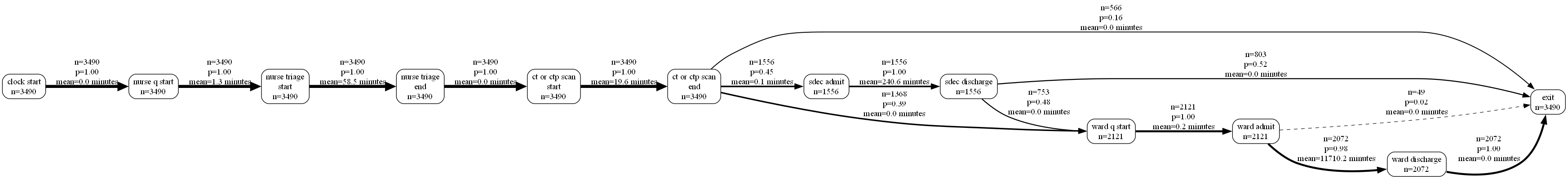

We can also change the orientation of the output.

dfg_to_graphviz(
    nodes,
    edges,
    min_frequency=5,
    direction="TD"
)

While the early parts of the process are easy to interpret in minutes, it’s hard to interpret the ward stay durations, which are much longer.

We might actually want to split these into two separate graphs by filtering the node and edges table.

For now, though, we’re going to rediscover our dfg using a unit of days, recalculate our timestamp and node/edge dataframes, and visualise this again. Note where ‘minutes’ has changed to ‘days’.

nodes, edges = discover_dfg(stroke_df_timestamp, case_col="id", time_unit="days")

dfg_to_graphviz(
    nodes,
    edges,
    min_frequency=5,
    time_unit="days",
)

Looping through graphviz outputs

While a lot of value can be obtained from just checking that your model is behaving as expected, you can get even more out of these outputs by faceting by different elements.

For example, here we expect patients with different stroke types to have different lengths of stay.

We need to import the display function from IPython.display and explicitly call this to ensure it’s included.

from IPython.display import display

for i in stroke_df_timestamp["patient_diagnosis_type"].unique():

    df = stroke_df_timestamp[stroke_df_timestamp["patient_diagnosis_type"]==i]

    nodes, edges = discover_dfg(df, case_col="id", time_unit="days")

    display(dfg_to_graphviz(
        nodes,
        edges,
        time_unit="days",
        title=f"Stroke Type: {i}"
    ))

We could do what we talked about earlier and try filtering the nodes and edges.

from IPython.display import display

for i in stroke_df_timestamp["patient_diagnosis_type"].unique():

    df = stroke_df_timestamp[stroke_df_timestamp["patient_diagnosis_type"]==i]

    nodes, edges = discover_dfg(df, case_col="id", time_unit="days")

    # Remember that we will need to include the newline indicator when filtering; we can work out where this is by visually observing
    # the node labels in the orignal diagram
    steps_to_include = ["ct or ctp scan\nend", "sdec admit", "sdec discharge", "ward q start", "ward admit", "ward discharge", "exit"]

    nodes = nodes[nodes["activity"].isin(steps_to_include)]

    edges = edges[(edges["source"].isin(steps_to_include)) |
                  (edges["target"].isin(steps_to_include))]

    display(dfg_to_graphviz(
        nodes,
        edges,
        time_unit="days",
        title=f"Stroke Type: {i}"
    ))

We could check out the maximum durations too.

for i in stroke_df_timestamp["patient_diagnosis_type"].unique():

    df = stroke_df_timestamp[stroke_df_timestamp["patient_diagnosis_type"]==i]

    nodes, edges = discover_dfg(df, case_col="id", time_unit="days")

    display(dfg_to_graphviz(
        nodes,
        edges,
        time_unit="days",
        title=f"Stroke Type: {i}",
        time_metric="max"
    ))

Interactive outputs

Finally, let’s take a look at an interactive output.

Here, we pass in the same nodes and edges. However, we need to choose a layout; ‘dagre’ is often the best option for getting something that looks similar to graphviz.

nodes, edges = discover_dfg(stroke_df_timestamp, case_col="id", timestamp_col="timestamp", time_unit="days")

op = dfg_to_cytoscape(
    nodes,
    edges,
    layout_name='dagre',
    layout_orientation="LR",
    spacing_factor=1.5,
    width=1400,
    time_unit="days")


display(op)

You can also try this out in the following Streamlit app.