from lokigi.site import SiteProblem
from lokigi.multiobjective import MetricMultiple Travel Matrices
Sometimes we want to weigh up more than one travel mode at once – for example, how a set of sites performs for car travel and for public transport, in a single ranked list of candidate solutions.
The ‘comparing solutions’ example shows how to do this by solving the same problem twice (once per mode, via problem.copy()) and then reconciling the two independently-ranked SiteSolutionSets with SolutionComparator. That approach is the right one when the two modes genuinely need separate optimisations – but the two solution sets are ranked over different orderings, and SolutionComparator.find_balanced_solution() can only reconcile them heuristically, by scoring how much their selected sites overlap.
This example instead registers public transport as a secondary travel matrix on a single problem. The primary matrix (car) still drives which combinations of sites get searched and pruned, but every solution solve() returns also carries public transport metrics alongside the car ones – so we get one ranked list, with both modes’ numbers side by side, ready to trade off directly with a Pareto front.
As with the comparing solutions example, we’ll use the Devon minor injury unit sites, but this time we only need a single SiteProblem – we don’t need to .copy() it per mode.
problem = SiteProblem()

problem.add_sites(
    "../../../sample_data/devon_mius.geojson",
    candidate_id_col="Facility_Name"
    )

problem.add_region_geometry_layer(
    "https://github.com/hsma-programme/h6_3c_interactive_plots_travel/raw/main/h6_3c_interactive_plots_travel/example_code/LSOA_2011_Boundaries_Super_Generalised_Clipped_BSC_EW_V4.geojson",
    common_col="LSOA11NM"
    )
Now we add our primary travel matrix – car – exactly as usual, via add_travel_matrix(). This is the matrix that solve() will optimise against.
problem.add_travel_matrix(
    travel_matrix_df="../../../sample_data/devon_miu_travel_matrix.csv",
    source_col="from_id",
    unit="minutes",
    )
Then we register public transport as a secondary travel matrix via add_secondary_travel_matrix(). It takes the same travel_matrix_df/source_col/unit arguments as add_travel_matrix(), plus a required label (used to name every metric column this matrix contributes) and an optional per-matrix threshold_for_coverage – public transport journeys are typically slower, so we’ll use a more generous 60-minute threshold here, independent of whatever threshold we pass to solve() for the primary (car) matrix.
You can register as many secondary matrices as you like this way – each one just needs its own unique label.
problem.add_secondary_travel_matrix(
    travel_matrix_df="../../../sample_data/devon_miu_travel_matrix_public_transport_extended.csv",
    source_col="from_id",
    label="public_transport",
    unit="minutes",
    threshold_for_coverage=60,
    )
Now we solve once. The threshold_for_coverage=20 here only applies to the primary (car) matrix, since public transport already has its own threshold of 60 minutes set at registration time above.
solution = problem.solve(p=4, threshold_for_coverage=20)/__w/lokigi/lokigi/lokigi/site.py:1177: UserWarning:
No demand data was provided. Demand from all regions has been assumed to be equal.If you wish to override this, run .add_demand() to add your site dataframe before running .solve() again.You can use the .show_demand_format() to see the expected format beforehand.
Let’s look at the column names now available. Alongside the usual car-based metrics (weighted_average, max, proportion_within_coverage_threshold, …), every one of those core metrics now also has a public_transport-suffixed sibling.
solution.show_solutions_colnames()Index(['solution_rank', 'site_names', 'site_indices', 'unselected_site_names',
'coverage_threshold', 'weighted_average', 'unweighted_average',
'90th_percentile', 'max', 'weighted_average_for_ranking',
'unweighted_average_for_ranking', 'max_for_ranking', 'total_cost',
'proportion_within_coverage_threshold',
'proportion_regions_within_coverage_threshold',
'demand_within_coverage_threshold', 'regions_within_coverage_threshold',
'regions_unreachable', 'demand_unreachable',
'proportion_demand_unreachable', 'weighted_by_equity_group',
'unweighted_by_equity_group', 'coverage_by_equity_group',
'coverage_regions_by_equity_group', 'max_cost_by_equity_group',
'regions_unreachable_by_equity_group',
'demand_unreachable_by_equity_group', 'gap_absolute_weighted',
'gap_relative_weighted', 'avg_lower_third_bins',
'avg_middle_third_bins', 'avg_upper_third_bins', 'inter_tertile_ratio',
'gap_absolute_description', 'gap_relative_description',
'inter_tertile_description', 'problem_df',
'weighted_average__public_transport',
'unweighted_average__public_transport',
'90th_percentile__public_transport', 'max__public_transport',
'proportion_within_coverage_threshold__public_transport',
'proportion_regions_within_coverage_threshold__public_transport',
'demand_within_coverage_threshold__public_transport',
'regions_within_coverage_threshold__public_transport',
'regions_unreachable__public_transport',
'demand_unreachable__public_transport',
'proportion_demand_unreachable__public_transport',
'gap_absolute_weighted__public_transport',
'gap_relative_weighted__public_transport',
'avg_lower_third_bins__public_transport',
'avg_middle_third_bins__public_transport',
'avg_upper_third_bins__public_transport',
'inter_tertile_ratio__public_transport'],
dtype='str')solution.show_solutions().head()| solution_rank | site_names | site_indices | unselected_site_names | coverage_threshold | weighted_average | unweighted_average | 90th_percentile | max | weighted_average_for_ranking | ... | regions_within_coverage_threshold__public_transport | regions_unreachable__public_transport | demand_unreachable__public_transport | proportion_demand_unreachable__public_transport | gap_absolute_weighted__public_transport | gap_relative_weighted__public_transport | avg_lower_third_bins__public_transport | avg_middle_third_bins__public_transport | avg_upper_third_bins__public_transport | inter_tertile_ratio__public_transport | |
|---|---|---|---|---|---|---|---|---|---|---|---|---|---|---|---|---|---|---|---|---|---|
| 0 | 1 | [North Devon District Hospital, Totnes Communi... | [0, 6, 7, 11] | [Honiton Hospital, Tiverton & District Hospita... | 20 | 20.23 | 20.23 | 33.0 | 64.0 | 20.23 | ... | 292 | 0 | 0.0 | 0.0 | None | None | None | None | None | None |
| 1 | 2 | [North Devon District Hospital, Newton Abbot C... | [0, 5, 7, 11] | [Honiton Hospital, Tiverton & District Hospita... | 20 | 20.68 | 20.68 | 34.4 | 64.0 | 20.68 | ... | 289 | 0 | 0.0 | 0.0 | None | None | None | None | None | None |
| 2 | 3 | [Totnes Community Hospital, NHS Walk in Centre... | [6, 7, 11, 13] | [North Devon District Hospital, Honiton Hospit... | 20 | 20.91 | 20.91 | 34.0 | 68.0 | 20.91 | ... | 270 | 0 | 0.0 | 0.0 | None | None | None | None | None | None |
| 3 | 4 | [North Devon District Hospital, Totnes Communi... | [0, 6, 7, 10] | [Honiton Hospital, Tiverton & District Hospita... | 20 | 21.10 | 21.10 | 34.0 | 64.0 | 21.10 | ... | 285 | 0 | 0.0 | 0.0 | None | None | None | None | None | None |
| 4 | 5 | [Totnes Community Hospital, NHS Walk in Centre... | [6, 7, 11, 12] | [North Devon District Hospital, Honiton Hospit... | 20 | 21.16 | 21.16 | 37.4 | 70.0 | 21.16 | ... | 279 | 0 | 0.0 | 0.0 | None | None | None | None | None | None |
5 rows × 54 columns
Exploring the trade-off with a Pareto front
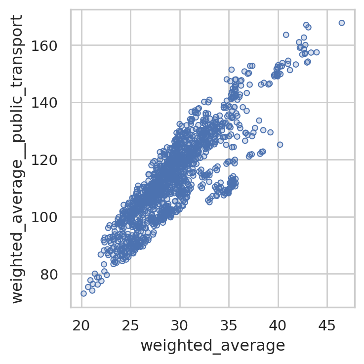
Because both modes’ metrics live on the same ranked list, we can trade them off directly with the same Pareto tooling used for e.g. cost vs equity in the Pareto fronts example – there’s nothing secondary-matrix-specific about compute_pareto_front() or plot_simple_pareto_front_pairs(), they just consume whichever solution_df columns you point them at.
solution.plot_simple_pareto_front_pairs(
    x_axis="weighted_average",
    y_axis="weighted_average__public_transport",
    )
We can bring in more metrics at once with Metric – here, car weighted average travel time, public transport weighted average travel time, and public transport coverage.
metrics = [
    Metric(column="weighted_average", direction="lower_better",
                 label="car weighted average travel time", unit="minutes"),
    Metric(column="weighted_average__public_transport", direction="lower_better",
                 label="public transport weighted average travel time", unit="minutes"),
    Metric(column="proportion_within_coverage_threshold__public_transport", direction="higher_better",
                 label="public transport coverage"),
    Metric(column="max__public_transport", direction="lower_better",
                 label="public transport max travel time", unit="minutes"),
    ]

solution.compute_pareto_front(metrics=metrics)

solution.pareto_summary()| solution_rank | weighted_average | weighted_average__public_transport | proportion_within_coverage_threshold__public_transport | max__public_transport | |
|---|---|---|---|---|---|
| 0 | 1 | 20.227723 | 73.074965 | 0.413013 | 294.0 |
| 1 | 12 | 22.260255 | 91.759547 | 0.294201 | 288.0 |
| 2 | 16 | 22.367751 | 92.676096 | 0.289958 | 281.0 |
| 3 | 18 | 22.643564 | 88.555870 | 0.298444 | 266.0 |
| 4 | 19 | 22.649222 | 87.267327 | 0.302687 | 266.0 |
| 5 | 34 | 23.261669 | 84.906648 | 0.381895 | 262.0 |
| 6 | 43 | 23.403112 | 84.260255 | 0.373409 | 262.0 |
| 7 | 172 | 25.390382 | 88.647808 | 0.417256 | 337.0 |
solution.plot_pareto_summary(width_multiplier=3);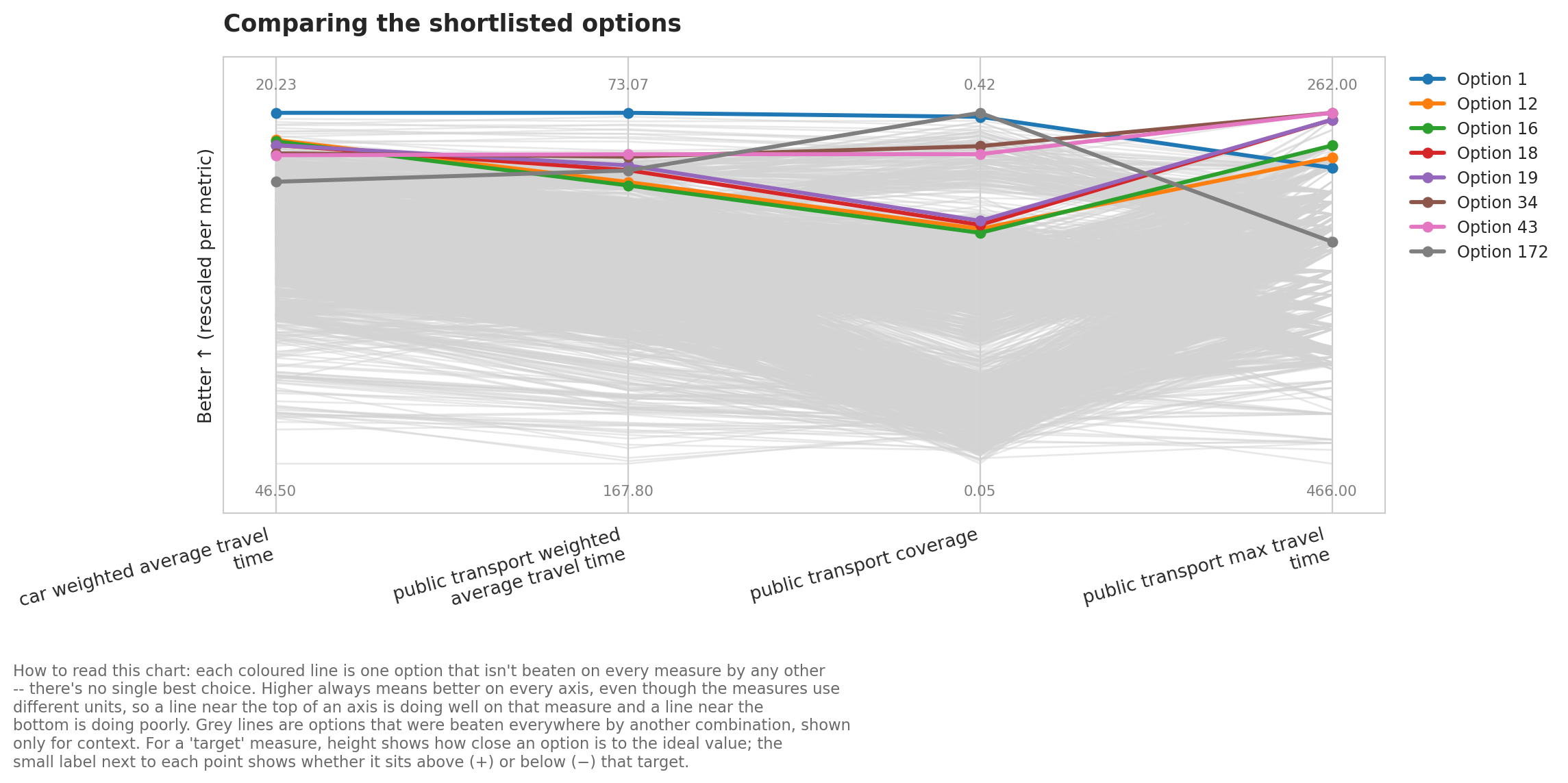
solution.plot_pareto_facets();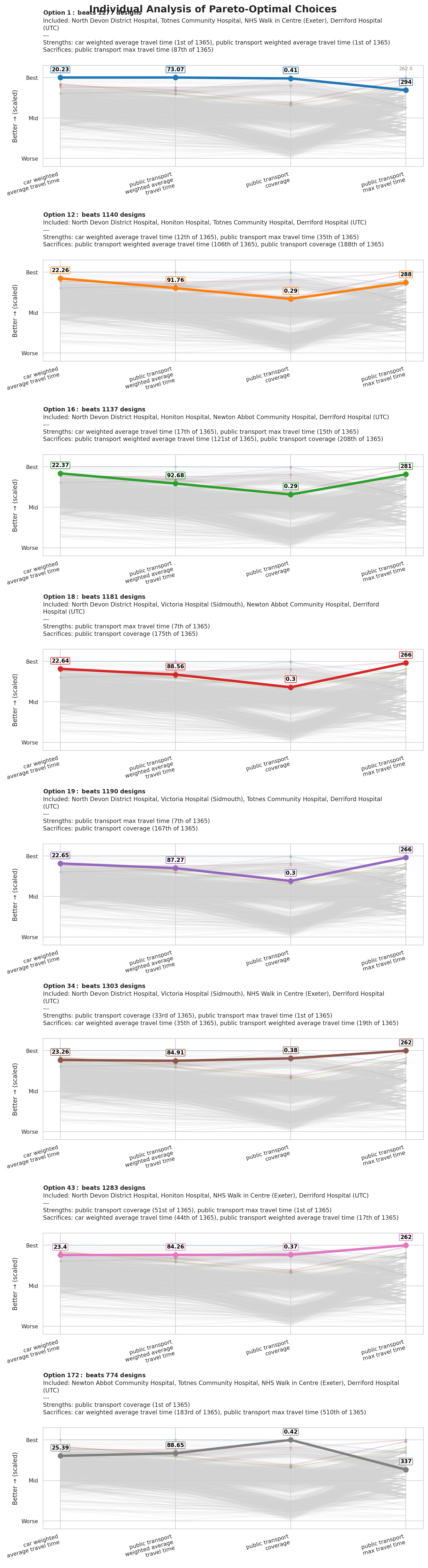
Plotting a secondary matrix directly
Every travel-related plot accepts a matrix= keyword to switch from the primary (car) matrix to a registered secondary one. For example, here’s the public transport travel time distribution for the best car-ranked solution, instead of its car travel times:
solution.plot_travel_time_distribution(matrix="public_transport", top_n=1)The same matrix= keyword works on plot_best_combination(), plot_n_best_combinations(), plot_solution_comparison(), check_solution_equity(), plot_top_n_solution_equity(), and plot_combination_by_equity().
Maps
This ability to specify the matrix also applies to map plots.
If we do not pass a matrix argument, it will default to the primary travel matrix.
Car
solution.plot_best_combination();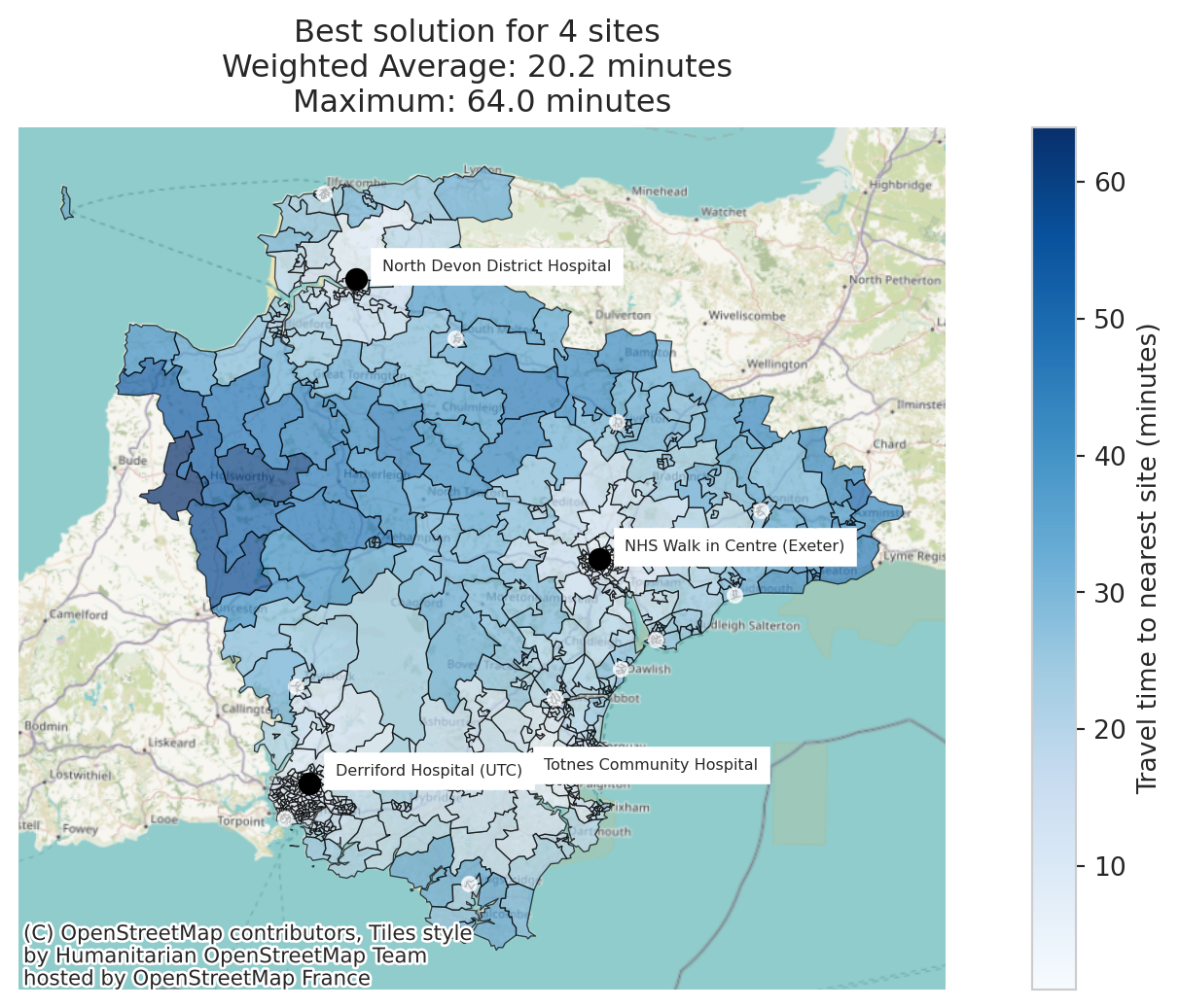
Public Transport
solution.plot_best_combination(matrix="public_transport");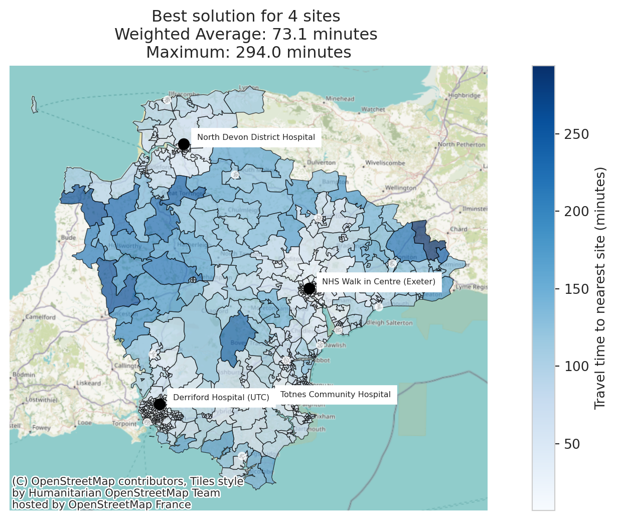
Ranking on a secondary matrix
Because weighted_average__public_transport is just another solution_df column, it can be used anywhere a column name is accepted – including sort_by, to re-sort the existing set of solutions by public transport performance instead of car performance.
solution.return_best_combination_site_names(sort_by="weighted_average__public_transport")['North Devon District Hospital',
'Totnes Community Hospital',
'NHS Walk in Centre (Exeter)',
'Derriford Hospital (UTC)']A caveat worth knowing about: sort_by only re-sorts the candidates that solve() already searched and kept. If you ran solve(..., brute_force_keep_best_n=...), discarded combinations were pruned using car performance alone – so a public_transport-ranked result over what survives is not necessarily the true best combination for public transport. When you’re planning to explore secondary-matrix trade-offs, it’s safest to solve with every combination retained (the default, or brute_force_keep_best_n=None), exactly as we’ve done in this example.
Handling genuinely unreachable journeys
Look again at the public transport matrix registered above – some of its values are 9999:
problem.show_secondary_travel_matrix("public_transport").drop(columns="from_id").max().sort_values(ascending=False).head()Honiton Hospital 9999.0
South Hams Hospital (Kingsbridge) 9999.0
Ilfracombe & District Tyrrell Hospital 543.0
Totnes Community Hospital 536.0
North Devon District Hospital 515.0
dtype: float649999 here is a sentinel: whoever generated this matrix used it to mean “no public transport route found” for a handful of origin-destination pairs, rather than leaving those cells empty – a common workaround, since add_secondary_travel_matrix() used to reject missing values outright. The problem is that 9999 isn’t actually excluded from anything downstream – it’s just a very large, very wrong number that every average, maximum, and map colour scale treats as a real 12+ hour journey.
Watch what it does to a single-site solution built around South Hams Hospital, the site with the most 9999s:
corrupted = problem.evaluate_baseline(
    site_names=["South Hams Hospital (Kingsbridge)"], threshold_for_coverage=20
    )
corrupted.solution_df[["weighted_average__public_transport", "max__public_transport"]]| weighted_average__public_transport | max__public_transport | |
|---|---|---|
| 0 | 732.165488 | 9999.0 |
A demand-weighted average public transport journey of over 12 hours, and a reported maximum of exactly 9999 – neither is a real travel time; both are the sentinel leaking into metrics that are supposed to describe actual journeys.
The fix: allow_missing and treat_as_missing
add_secondary_travel_matrix() (and add_travel_matrix() for a primary matrix) accepts allow_missing=True to register a matrix that genuinely has no feasible journey for some pairs, and treat_as_missing=<value> to convert an existing sentinel like 9999 to a proper missing value first. Missing values are then treated as “no feasible journey” throughout – excluded from every average/maximum, and rendered as a distinct grey region on maps, rather than either crashing or silently corrupting the numbers.
Since a label can only be registered once per problem, we register a fresh SiteProblem with the corrected registration (the sites/region-layer/car-matrix setup is identical to the top of this notebook):
problem_honest = SiteProblem()

problem_honest.add_sites(
    "../../../sample_data/devon_mius.geojson",
    candidate_id_col="Facility_Name"
    )

problem_honest.add_region_geometry_layer(
    "https://github.com/hsma-programme/h6_3c_interactive_plots_travel/raw/main/h6_3c_interactive_plots_travel/example_code/LSOA_2011_Boundaries_Super_Generalised_Clipped_BSC_EW_V4.geojson",
    common_col="LSOA11NM"
    )

problem_honest.add_travel_matrix(
    travel_matrix_df="../../../sample_data/devon_miu_travel_matrix.csv",
    source_col="from_id",
    unit="minutes",
    )

problem_honest.add_secondary_travel_matrix(
    travel_matrix_df="../../../sample_data/devon_miu_travel_matrix_public_transport_extended.csv",
    source_col="from_id",
    label="public_transport",
    unit="minutes",
    threshold_for_coverage=60,
    allow_missing=True,
    treat_as_missing=9999,
    )
Evaluating the same single-site solution now gives an honest average – computed only over regions that can actually reach the site by public transport – alongside an explicit count of how many, and how much demand, couldn’t:
honest = problem_honest.evaluate_baseline(
    site_names=["South Hams Hospital (Kingsbridge)"], threshold_for_coverage=20
    )
honest.solution_df[[
    "weighted_average__public_transport",
    "max__public_transport",
    "regions_unreachable__public_transport",
    "demand_unreachable__public_transport",
    "proportion_demand_unreachable__public_transport",
    ]]
/__w/lokigi/lokigi/lokigi/site.py:647: UserWarning:
No demand data was provided. Demand from all regions has been assumed to be equal. If you wish to override this, run .add_demand() to add your demand dataframe before calling evaluate_baseline() again.
| weighted_average__public_transport | max__public_transport | regions_unreachable__public_transport | demand_unreachable__public_transport | proportion_demand_unreachable__public_transport | |
|---|---|---|---|---|---|
| 0 | 191.137725 | 399.0 | 39 | 39.0 | 0.055163 |
191 minutes and a maximum of 399 – both real, honest journey times – plus an explicit “39 of 707 regions (5.5% of assumed-equal demand) have no public transport route at all” that used to be invisible, baked silently into a nonsensical 732-minute average.
The map reflects the same honesty: unreachable regions are shaded a distinct grey rather than left an unexplained hole, and the title states the count directly.
honest.plot_best_combination(matrix="public_transport", show_all_locations=False);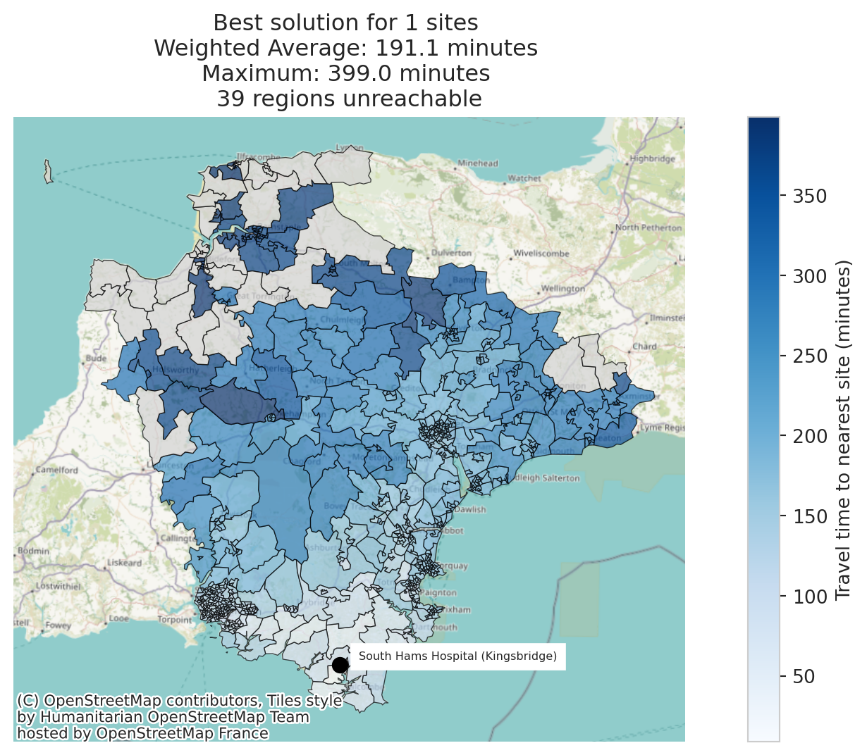
When would you actually use this? Public transport (or walking/cycling) matrices are usually generated with a permissive search radius/time limit to keep generation fast – see obtaining travel time matrices – which means some pairs genuinely have no route within that limit. allow_missing/treat_as_missing let you register that matrix as-is instead of widening the search (slow) or inventing a sentinel (corrupting). If the primary matrix (the one solve() optimises against, car in this example) has missing values, solve() additionally requires unreachable_cost=<a number> – a cost assumed for unreachable pairs only when ranking/pruning combinations, never in the reported metrics above – since otherwise a combination could be silently rewarded for stranding demand behind an unreachable pair. Secondary matrices, as used here, never drive optimisation, so no such policy is needed.
Which approach should I use?
- Secondary travel matrices (this example): one
solve(), one ranked list, with every registered matrix’s metrics available side by side. Best when you want to explore trade-offs between modes for the same candidate solutions – e.g. with a Pareto front. problem.copy()+SolutionComparator(see the comparing solutions example): two independent solves, each optimised (and pruned) entirely on its own mode. Best when the two modes genuinely need separate optimisations – e.g. very different candidate site sets, capacities, or objectives per mode – and you wantfind_balanced_solution()’s rank-overlap heuristic to reconcile them afterwards.