Site location problems without geometry and mapping

Lokigi can also support answering site location problems with a very minimal dataset - just the travel matrix, in fact!

However, here we’re also going to pass in a demand matrix as we know how much demand is coming from each location. However, the site names we’ve been given and the postcode sector names have been anonymised, so we are unable to map them back to an actual geographical region that we can plot.

from lokigi.site import SiteProblem

First, let’s initialise our SiteProblem() and add the demand and travel data.

Note

The data for this problem comes from github.com/health-data-science-OR/healthcare-logistics and is reused under the MIT licence.

Credit for the creation of this dataset goes to Dr Tom Monks.

Click here to view the licence for this dataset

MIT License

Copyright (c) 2020 health-data-science-OR

Permission is hereby granted, free of charge, to any person obtaining a copy
of this software and associated documentation files (the "Software"), to deal
in the Software without restriction, including without limitation the rights
to use, copy, modify, merge, publish, distribute, sublicense, and/or sell
copies of the Software, and to permit persons to whom the Software is
furnished to do so, subject to the following conditions:

The above copyright notice and this permission notice shall be included in all
copies or substantial portions of the Software.

THE SOFTWARE IS PROVIDED "AS IS", WITHOUT WARRANTY OF ANY KIND, EXPRESS OR
IMPLIED, INCLUDING BUT NOT LIMITED TO THE WARRANTIES OF MERCHANTABILITY,
FITNESS FOR A PARTICULAR PURPOSE AND NONINFRINGEMENT. IN NO EVENT SHALL THE
AUTHORS OR COPYRIGHT HOLDERS BE LIABLE FOR ANY CLAIM, DAMAGES OR OTHER
LIABILITY, WHETHER IN AN ACTION OF CONTRACT, TORT OR OTHERWISE, ARISING FROM,
OUT OF OR IN CONNECTION WITH THE SOFTWARE OR THE USE OR OTHER DEALINGS IN THE
SOFTWARE.

problem = SiteProblem()

problem.add_demand("https://github.com/health-data-science-OR/healthcare-logistics/blob/master/optimisation/data/sh_demand.csv", demand_col="n_patients", location_id_col="sector")

problem.show_demand()

	sector	n_patients
0	PS1	3375
1	PS2	3338
2	PS3	2922
3	PS4	3191
4	PS5	3134
...	...	...
273	PS274	216
274	PS275	261
275	PS276	342
276	PS277	0
277	PS278	0

278 rows × 2 columns

problem.add_travel_matrix(
    "https://github.com/health-data-science-OR/healthcare-logistics/blob/master/optimisation/data/clinic_car_travel_time.csv",
    source_col="sector"
    )

problem.show_travel_matrix()

	sector	clinic_1	clinic_2	clinic_3	clinic_4	clinic_5	clinic_6	clinic_7	clinic_8	clinic_9	...	clinic_19	clinic_20	clinic_21	clinic_22	clinic_23	clinic_24	clinic_25	clinic_26	clinic_27	clinic_28
0	PS158	33.17	40.15	38.17	37.93	29.35	51.48	53.28	48.00	53.82	...	12.10	12.27	15.83	53.27	53.98	29.75	34.22	32.68	19.62	39.25
1	PS159	31.42	36.55	36.42	34.53	27.60	47.88	49.68	44.40	50.22	...	11.75	11.92	10.62	49.68	50.38	26.15	30.62	32.35	19.28	35.65
2	PS160	31.82	38.80	36.82	36.58	28.00	50.13	51.95	46.65	52.47	...	10.75	10.92	14.35	51.93	52.65	28.40	32.87	31.35	18.27	37.90
3	PS161	31.68	38.65	36.67	36.43	27.87	49.98	51.80	46.50	52.32	...	10.32	10.77	16.38	51.78	52.50	28.27	32.73	31.20	17.82	37.75
4	PS162	29.55	36.53	34.55	34.32	25.73	47.87	49.67	44.38	50.20	...	6.77	7.28	17.18	49.65	50.37	26.13	30.60	29.07	14.27	35.63
...	...	...	...	...	...	...	...	...	...	...	...	...	...	...	...	...	...	...	...	...	...
273	PS273	34.13	21.83	39.23	35.90	34.70	49.25	49.08	45.78	51.58	...	54.62	53.95	43.67	51.05	3.85	28.45	28.67	42.50	52.72	22.15
274	PS157	29.60	17.30	34.70	31.37	30.17	44.72	44.55	41.25	47.05	...	51.27	50.60	40.32	46.52	6.22	27.22	24.13	37.95	49.38	17.62
275	PS274	31.17	18.38	36.28	32.95	31.73	46.30	46.13	42.82	48.63	...	49.03	48.35	38.08	48.10	8.25	22.10	25.72	37.57	47.13	18.70
276	PS275	34.40	23.73	39.40	37.52	30.58	50.87	52.68	47.38	53.20	...	47.82	47.13	36.87	52.67	12.30	22.65	32.75	36.35	45.92	25.22
277	PS276	37.80	25.52	42.90	39.58	38.37	52.93	52.77	49.45	55.27	...	58.32	57.65	47.38	54.73	11.17	32.48	32.35	46.17	56.43	25.82

278 rows × 29 columns

Now, we’ll solve this for 3 possible sites.

solution_3 = problem.solve(p=3, objectives="p_median", show_brute_force_progress=True)

/__w/lokigi/lokigi/lokigi/site.py:1378: UserWarning: No candidate site dataframe was given.
Sites names have been taken from the columns of your travel matrix: clinic_1, clinic_2, clinic_3, clinic_4, clinic_5, clinic_6, clinic_7, clinic_8, clinic_9, clinic_10, clinic_11, clinic_12, clinic_13, clinic_14, clinic_15, clinic_16, clinic_17, clinic_18, clinic_19, clinic_20, clinic_21, clinic_22, clinic_23, clinic_24, clinic_25, clinic_26, clinic_27, clinic_28.
If you wish to override this, run .add_sites() to add your site dataframe before running .solve() again.
You can use the .show_sites_format() to see the expected format beforehand.
  warn(

We can see that lokigi has warned us that we didn’t pass in a candidate site dataframe. As we didn’t have anything extra we wanted to pass in for our sites, like their exact locations or whether certain sites had to be included in the solution, this is fine.

If we want, we can see what site dataframe lokigi has automatically created.

problem.show_sites()

	index	site
0	0	clinic_1
1	1	clinic_2
2	2	clinic_3
3	3	clinic_4
4	4	clinic_5
5	5	clinic_6
6	6	clinic_7
7	7	clinic_8
8	8	clinic_9
9	9	clinic_10
10	10	clinic_11
11	11	clinic_12
12	12	clinic_13
13	13	clinic_14
14	14	clinic_15
15	15	clinic_16
16	16	clinic_17
17	17	clinic_18
18	18	clinic_19
19	19	clinic_20
20	20	clinic_21
21	21	clinic_22
22	22	clinic_23
23	23	clinic_24
24	24	clinic_25
25	25	clinic_26
26	26	clinic_27
27	27	clinic_28

Now let’s look at our solutions.

solution_3.show_solutions()

	site_names	site_indices	coverage_threshold	weighted_average	unweighted_average	90th_percentile	max	proportion_within_coverage_threshold	problem_df
0	None	[0, 7, 11]	None	11.12	14.57	26.78	36.18	0.0	sector sector_x clinic_1 clinic_8 clini...
1	None	[0, 9, 11]	None	11.37	14.63	26.89	36.18	0.0	sector sector_x clinic_1 clinic_10 clin...
2	None	[4, 7, 11]	None	11.51	14.45	25.52	32.37	0.0	sector sector_x clinic_5 clinic_8 clini...
3	None	[0, 11, 21]	None	11.56	15.17	27.11	36.18	0.0	sector sector_x clinic_1 clinic_12 clin...
4	None	[0, 8, 11]	None	11.58	15.23	27.25	36.18	0.0	sector sector_x clinic_1 clinic_9 clini...
...	...	...	...	...	...	...	...	...	...
3271	None	[13, 17, 19]	None	35.23	29.30	45.23	54.35	0.0	sector sector_x clinic_14 clinic_18 cli...
3272	None	[13, 17, 18]	None	35.51	29.53	45.70	54.35	0.0	sector sector_x clinic_14 clinic_18 cli...
3273	None	[17, 18, 19]	None	35.83	30.34	45.74	54.35	0.0	sector sector_x clinic_18 clinic_19 cli...
3274	None	[13, 18, 19]	None	36.13	30.03	46.66	57.93	0.0	sector sector_x clinic_14 clinic_19 cli...
3275	None	[18, 19, 26]	None	42.30	41.74	61.69	68.77	0.0	sector sector_x clinic_19 clinic_20 cli...

3276 rows × 9 columns

Plots you can still do when you have no geometry

There are still a number of different useful plots you can create when you don’t have a geometry layer.

Bar chart of best combinations

solution_3.plot_n_best_combinations_bar()

We can adjust the number of combinations shown.

solution_3.plot_n_best_combinations_bar(n_best=5)

And compare or rank on different things.

solution_3.plot_n_best_combinations_bar(y_axis="max")

solution_3.plot_n_best_combinations_bar(y_axis="max", rank_on="max")

Pareto fronts

Pareto front plots help us to understand tradeoffs between different objectives.

By default, the single pareto plot will compare weighted average travel time to the max travel time of each solution.

solution_3.plot_simple_pareto_front()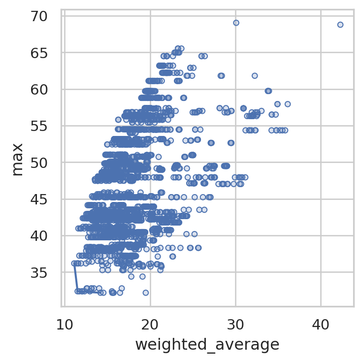

We can change what it’s plotting.

solution_3.plot_simple_pareto_front(y_axis="90th_percentile")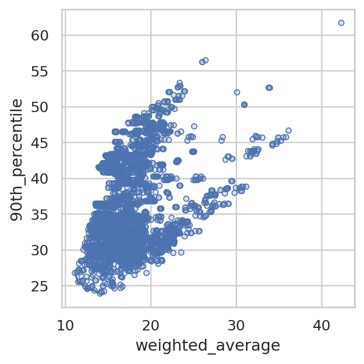

We can hide the individual points if the pareto front is hard to see.

solution_3.plot_simple_pareto_front(y_axis="90th_percentile", show_points=False)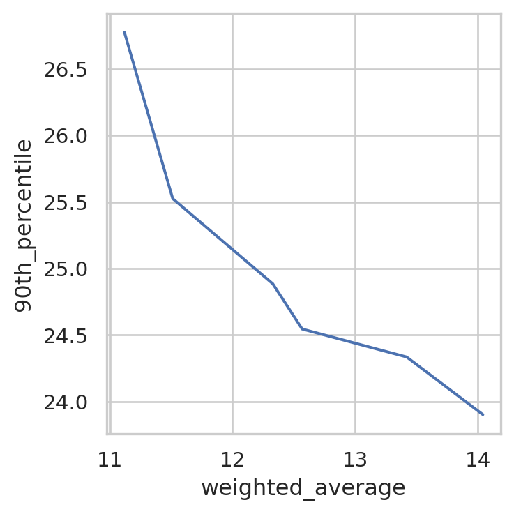

We can also ask it to create a plot of every pair of metrics.

solution_3.plot_all_metric_pareto_front()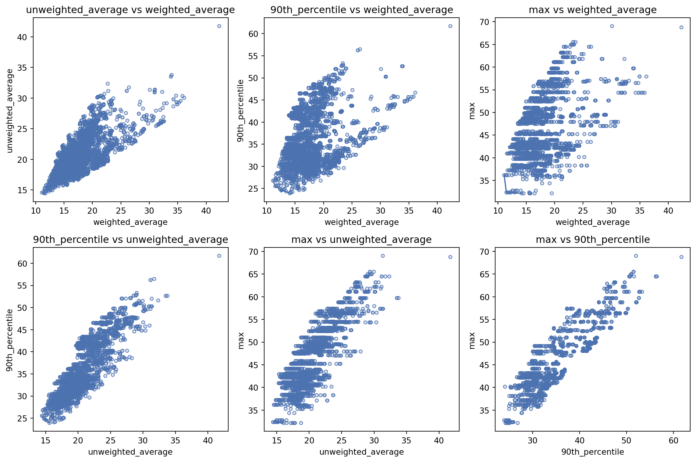

Travel time distribution

Let’s take a quick look at how much the travel time varied for our best solution.

solution_3.plot_travel_time_distribution()

How did the top 5 compare?

solution_3.plot_travel_time_distribution(top_n=5)

We can visualise the differences per region more easily by setting compare_to_best=True.

solution_3.plot_travel_time_distribution(top_n=5, compare_to_best=True)