Minimizing the average travel time to sites

First, we need to import and initialise the SiteProblem class.

from lokigi.site import SiteProblem
import pandas as pd

problem = SiteProblem()

Let’s see what models are currently supported.

problem.describe_models(available_only=True)

=== Supported Healthcare Location Models ===

ID: simple_p_median
Name: P-Median (Average Distance Minimizer)
Goal: Minimize the total travel distance or time.
When to use: Best for situations like siting a series of storage hubs efficiently across a region where demand/volume doesn't matter.
Main Trade-off: Can leave remote or rural patients with very long travel times in favor of urban density.

ID: p_median
Name: P-Median (Average Weighted Distance Minimizer)
Goal: Minimize the total travel distance or time for the entire population, weighting the travel times by a metric such as demand per region.
When to use: Best for general primary care where you want the 'average' patient to have the shortest trip possible.
Main Trade-off: Can leave remote or rural patients with very long travel times in favor of urban density.

ID: hybrid_simple_p_median
Name: Hybrid Simple P-Median (The Safety Net Model)
Goal: Minimize the total travel distance or time, weighting the travel times by a metric such as demand per region, while guaranteeing a maximum 'cutoff' time for every patient.
When to use: Makes the system efficient while preventing major 'postcode lotteries' where some patients travel a very long way.
Main Trade-off: Hard cut-off point could see some good solutions that nearly meet the cutoff being discarded.

ID: hybrid_p_median
Name: Hybrid P-Median (The Safety Net Model)
Goal: Minimize average travel distance or time while guaranteeing a maximum 'cutoff' time for every patient.
When to use: Makes the system efficient while preventing major 'postcode lotteries' where some patients travel a very long way.
Main Trade-off: Hard cut-off point could see some good solutions that nearly meet the cutoff being discarded.

ID: p_center
Name: P-Center (The Fair-Maximum Model)
Goal: Minimize the maximum travel distance or time for the furthest patient.
When to use: Best for ensuring universal access in rural regions; 'No one left behind'.
Main Trade-off: Can lead to higher average travel distances or times for the majority population.

ID: mclp
Name: Maximal Coverage Location Problem (MCLP)
Goal: Maximize the number of people within a specific time/distance 'threshold' (e.g., 15 minutes).
When to use: Best for emergency services (Ambulance/ER) where getting there within a 'Golden Hour' is more important than the average trip time.
Main Trade-off: Does not care how far away people are once they are outside the threshold.

To run a model, use: prob.solve_pmedian(p=3) or similar.

And what models will be supported in the future?

problem.describe_models(available_only=False)

=== Healthcare Location Models ===

ID: simple_p_median
Name: P-Median (Average Distance Minimizer)
Goal: Minimize the total travel distance or time.
When to use: Best for situations like siting a series of storage hubs efficiently across a region where demand/volume doesn't matter.
Main Trade-off: Can leave remote or rural patients with very long travel times in favor of urban density.
Status: Supported

ID: p_median
Name: P-Median (Average Weighted Distance Minimizer)
Goal: Minimize the total travel distance or time for the entire population, weighting the travel times by a metric such as demand per region.
When to use: Best for general primary care where you want the 'average' patient to have the shortest trip possible.
Main Trade-off: Can leave remote or rural patients with very long travel times in favor of urban density.
Status: Supported

ID: hybrid_simple_p_median
Name: Hybrid Simple P-Median (The Safety Net Model)
Goal: Minimize the total travel distance or time, weighting the travel times by a metric such as demand per region, while guaranteeing a maximum 'cutoff' time for every patient.
When to use: Makes the system efficient while preventing major 'postcode lotteries' where some patients travel a very long way.
Main Trade-off: Hard cut-off point could see some good solutions that nearly meet the cutoff being discarded.
Status: Supported

ID: hybrid_p_median
Name: Hybrid P-Median (The Safety Net Model)
Goal: Minimize average travel distance or time while guaranteeing a maximum 'cutoff' time for every patient.
When to use: Makes the system efficient while preventing major 'postcode lotteries' where some patients travel a very long way.
Main Trade-off: Hard cut-off point could see some good solutions that nearly meet the cutoff being discarded.
Status: Supported

ID: p_center
Name: P-Center (The Fair-Maximum Model)
Goal: Minimize the maximum travel distance or time for the furthest patient.
When to use: Best for ensuring universal access in rural regions; 'No one left behind'.
Main Trade-off: Can lead to higher average travel distances or times for the majority population.
Status: Supported

ID: mclp
Name: Maximal Coverage Location Problem (MCLP)
Goal: Maximize the number of people within a specific time/distance 'threshold' (e.g., 15 minutes).
When to use: Best for emergency services (Ambulance/ER) where getting there within a 'Golden Hour' is more important than the average trip time.
Main Trade-off: Does not care how far away people are once they are outside the threshold.
Status: Supported

ID: lscp
Name: Location Set Covering Location Problem (LSCP)
Goal: Find the minimum number of facilities needed to cover *everyone* within a certain distance.
When to use: Best for universal mandates (e.g., ensuring every citizen is within 20 miles of a pharmacy).
Main Trade-off: Can be very expensive as it forces clinics into sparsely populated areas to reach the final 1%.
Status: Planned

ID: lscp-b
Name: LSCP-B (Backup Coverage Model)
Goal: Minimize the number of facilities needed to ensure everyone is covered by AT LEAST TWO locations.
When to use: Critical for high-reliability services like Maternity units or Stroke centers where 'System Busy' is a life-threatening risk.
Main Trade-off: Requires significantly more resources (budget/staff) than standard coverage to achieve the same geographic footprint.
Status: Planned

To run a model, use: prob.solve_pmedian(p=3) or similar.

Initialising required data

The show_ methods help us to see what format lokigi expects our data to be in.

problem.show_demand_format()


--- Expected Demand DataFrame Format ---
Note: Each row represents a unique demand location (e.g., LSOA).
site_id_col     | demand_col
------------------------------
LSOA 1          | 25        
LSOA 2          | 15        
...             | ...       
----------------------------------------

problem.show_travel_format()


--- Expected Travel/Cost DataFrame Format ---
Note: Rows are sources, columns are destinations.
source_id       | dest_1          | dest_2         
--------------------------------------------------
source_1        | 22.6            | 16.3           
source_2        | 15.1            | 17.1           
...             | ...             | ...            
--------------------------------------------

For example, if using LSOAs, your dataframe might look like this:
source_id       | E01000259       | E01000314      
--------------------------------------------------
Brighton and Hove 027E | 22.6            | 16.3           
Brighton and Hove 005C | 15.1            | 17.1           
...             | ...             | ...            
--------------------------------------------

Or if you've defined your site names, it might look like this:
source_id       | Site 1          | Site 1         
--------------------------------------------------
Brighton and Hove 027E | 22.6            | 16.3           
Brighton and Hove 005C | 15.1            | 17.1           
...             | ...             | ...            
--------------------------------------------

Add the required data

We can now use the various add_ methods to add in the required datasets.

Historical Demand

problem.add_demand("../../../sample_data/brighton_demand.csv", demand_col="demand", location_id_col="LSOA")

problem.show_demand()

	LSOA	demand
0	Brighton and Hove 027E	3627
1	Brighton and Hove 027F	2323
2	Brighton and Hove 027A	2596
3	Brighton and Hove 029E	3132
4	Brighton and Hove 029D	2883
...	...	...
160	Brighton and Hove 012A	2497
161	Brighton and Hove 005C	2570
162	Brighton and Hove 012B	2051
163	Brighton and Hove 005A	1164
164	Brighton and Hove 005B	1097

165 rows × 2 columns

Candidate Sites

problem.add_sites("../../../sample_data/brighton_sites_named.geojson", candidate_id_col="site")

problem.show_sites()

	index	site	geometry
0	0	Dahlia (Site 1)	POINT (527142.275 106616.053)
1	1	Begonia (Site 2)	POINT (531493.995 106639.488)
2	2	Tulip (Site 3)	POINT (533356.778 105476.782)
3	3	Daisy (Site 4)	POINT (528513.424 105052.43)
4	4	Daffodil (Site 5)	POINT (532421.163 109069.196)
5	5	Snowdrop (Site 6)	POINT (528716.452 108042.794)

We can also plot the sites we’ve just put in.

problem.plot_sites()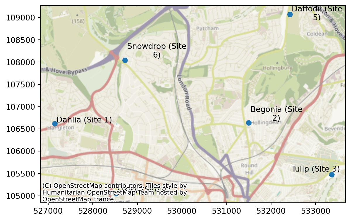

problem.plot_sites(interactive=True)

Make this Notebook Trusted to load map: File -> Trust Notebook

Travel Data

Our travel matrix is in seconds. Let’s update this to minutes when we load it in.

problem.add_travel_matrix(
    travel_matrix_df="../../../sample_data/brighton_travel_matrix_driving_named.csv",
    source_col="LSOA",
    from_unit="seconds",
    to_unit="minutes"
    )

problem.travel_matrix

	LSOA	Dahlia (Site 1)	Begonia (Site 2)	Tulip (Site 3)	Daisy (Site 4)	Daffodil (Site 5)	Snowdrop (Site 6)
0	Brighton and Hove 027E	12.898833	8.794833	7.404833	8.197500	10.125667	9.248500
1	Brighton and Hove 027F	12.623167	8.318500	8.626167	9.351167	9.649500	8.972833
2	Brighton and Hove 027A	12.720667	10.023000	8.633000	6.840000	11.353833	9.289167
3	Brighton and Hove 029E	12.393667	10.862000	11.006000	6.328667	12.193000	9.293000
4	Brighton and Hove 029D	11.097500	11.077500	10.970000	5.216667	12.408333	9.508500
...	...	...	...	...	...	...	...
160	Brighton and Hove 012A	7.442333	14.745000	18.468500	8.652667	10.433667	7.463000
161	Brighton and Hove 005C	7.830000	13.080500	16.804000	9.490000	8.769167	5.798500
162	Brighton and Hove 012B	7.742167	15.153000	18.876667	8.952500	10.841833	7.871000
163	Brighton and Hove 005A	9.458167	14.708667	18.432167	11.068500	10.397333	7.426667
164	Brighton and Hove 005B	8.258333	13.508833	17.232333	9.918333	9.197500	6.226833

165 rows × 7 columns

Region Geometry

We’ll also want to add in a region geometry layer (a geodataframe containing the boundaries for the areas defined in our demand data) if we want to be able to plot some of our outputs.

problem.add_region_geometry_layer("https://github.com/hsma-programme/h6_3d_facility_location_problems/raw/refs/heads/main/h6_3d_facility_location_problems/example_code/LSOA_2011_Boundaries_Super_Generalised_Clipped_BSC_EW_V4.geojson", common_col="LSOA11NM")

# problem.add_region_geometry_layer("../../../sample_data/LSOA_2011_Boundaries_Super_Generalised_Clipped_BSC_EW_V4.geojson", common_col="LSOA11NM")

problem.show_region_geometry_layer()

	FID	LSOA11CD	LSOA11NM	LSOA11NMW	BNG_E	BNG_N	LONG	LAT	GlobalID	geometry
0	1	E01000001	City of London 001A	City of London 001A	532123	181632	-0.097140	51.51816	a758442e-7679-45d0-95a8-ed4c968ecdaa	POLYGON ((532282.629 181906.496, 532248.25 181...
1	2	E01000002	City of London 001B	City of London 001B	532480	181715	-0.091970	51.51882	861dbb53-dfaf-4f57-be96-4527e2ec511f	POLYGON ((532746.814 181786.892, 532248.25 181...
2	3	E01000003	City of London 001C	City of London 001C	532239	182033	-0.095320	51.52174	9f765b55-2061-484a-862b-fa0325991616	POLYGON ((532293.068 182068.422, 532419.592 18...
3	4	E01000005	City of London 001E	City of London 001E	533581	181283	-0.076270	51.51468	a55c4c31-ef1c-42fc-bfa9-07c8f2025928	POLYGON ((533604.245 181418.129, 533743.689 18...
4	5	E01000006	Barking and Dagenham 016A	Barking and Dagenham 016A	544994	184274	0.089317	51.53875	9cdabaa8-d9bd-4a94-bb3b-98a933ceedad	POLYGON ((545271.918 184183.948, 545296.314 18...
...	...	...	...	...	...	...	...	...	...	...
34748	34749	W01001954	Cardiff 006F	Caerdydd 006F	312959	180574	-3.255820	51.51735	5fc2d16e-8663-462f-936d-7535d0de1732	POLYGON ((313011.929 181083.89, 313533.809 180...
34749	34750	W01001955	Swansea 025F	Abertawe 025F	265633	193182	-3.942370	51.62137	0bcc9472-48d1-460c-a40e-c4a745269d84	POLYGON ((266079.095 193572.406, 266140.774 19...
34750	34751	W01001956	Swansea 023E	Abertawe 023E	260586	192621	-4.015000	51.61510	557e08ba-6aee-491d-8ba1-79eca916ce6b	POLYGON ((260107.578 194891.58, 260436.897 194...
34751	34752	W01001957	Swansea 025G	Abertawe 025G	265337	192555	-3.946400	51.61567	43f945c4-e97d-4b1f-9e4d-46d154a6662e	POLYGON ((264991.859 192395.89, 264913.891 192...
34752	34753	W01001958	Swansea 025H	Abertawe 025H	266265	192630	-3.933030	51.61656	84055fe9-868f-4150-9bea-082777cf132d	POLYGON ((266566.301 192259, 266577.9 191916.2...

34753 rows × 10 columns

problem.plot_region_geometry_layer()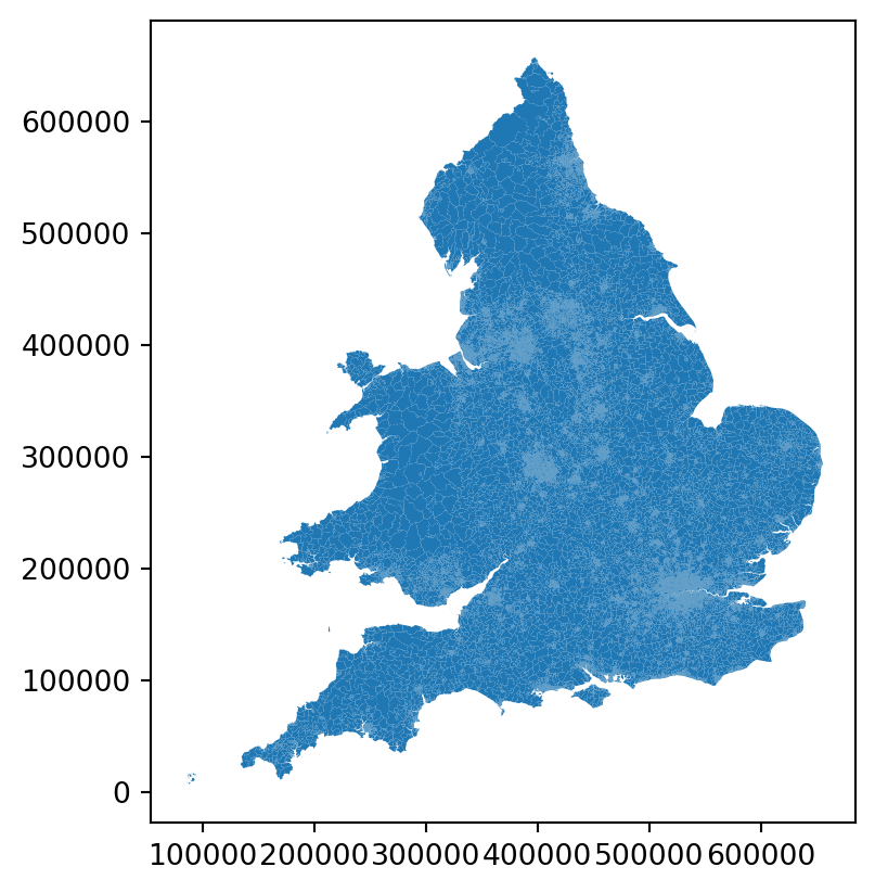

problem.plot_region_geometry_layer(plot_demand=True)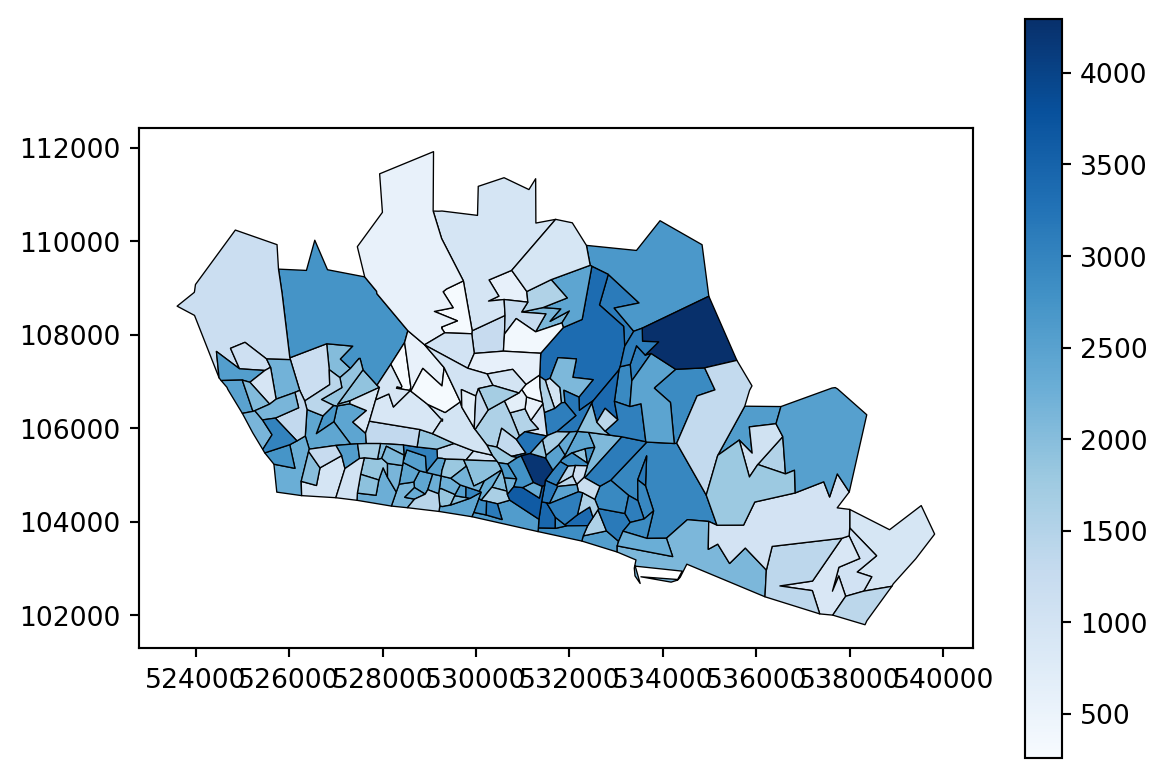

problem.plot_region_geometry_layer(interactive=True, height=600, width=600)

Make this Notebook Trusted to load map: File -> Trust Notebook

problem.plot_region_geometry_layer(interactive=True, plot_demand=True, height=600, width=600)

Make this Notebook Trusted to load map: File -> Trust Notebook

Evaluating a single solution

Generally we’re going to want to evaluate lots of solutions at once to find the optimum one.

However, we can also choose to evaluate a single solution.

combo_1 = problem.evaluate_single_solution_single_objective(site_names=["Dahlia (Site 1)", "Begonia (Site 2)"])
combo_1

<lokigi.site_solutions.EvaluatedCombination at 0x7f234dadbb30>

combo_1.return_solution_metrics()

{'site_names': ['Dahlia (Site 1)', 'Begonia (Site 2)'],
 'site_indices': array([0, 1]),
 'coverage_threshold': None,
 'weighted_average': np.float64(8.450685200470566),
 'unweighted_average': np.float64(8.152459595959595),
 '90th_percentile': np.float64(11.978799999999998),
 'max': np.float64(23.921),
 'proportion_within_coverage_threshold': np.float64(0.0),
 'problem_df':                        LSOA                  LSOA_x  Dahlia (Site 1)  \
 0    Brighton and Hove 027E  Brighton and Hove 027E        12.898833   
 1    Brighton and Hove 027F  Brighton and Hove 027F        12.623167   
 2    Brighton and Hove 027A  Brighton and Hove 027A        12.720667   
 3    Brighton and Hove 029E  Brighton and Hove 029E        12.393667   
 4    Brighton and Hove 029D  Brighton and Hove 029D        11.097500   
 ..                      ...                     ...              ...   
 160  Brighton and Hove 012A  Brighton and Hove 012A         7.442333   
 161  Brighton and Hove 005C  Brighton and Hove 005C         7.830000   
 162  Brighton and Hove 012B  Brighton and Hove 012B         7.742167   
 163  Brighton and Hove 005A  Brighton and Hove 005A         9.458167   
 164  Brighton and Hove 005B  Brighton and Hove 005B         8.258333   
 
      Begonia (Site 2)   min_cost     selected_site  within_threshold  \
 0            8.794833   8.794833  Begonia (Site 2)               NaN   
 1            8.318500   8.318500  Begonia (Site 2)               NaN   
 2           10.023000  10.023000  Begonia (Site 2)               NaN   
 3           10.862000  10.862000  Begonia (Site 2)               NaN   
 4           11.077500  11.077500  Begonia (Site 2)               NaN   
 ..                ...        ...               ...               ...   
 160         14.745000   7.442333   Dahlia (Site 1)               NaN   
 161         13.080500   7.830000   Dahlia (Site 1)               NaN   
 162         15.153000   7.742167   Dahlia (Site 1)               NaN   
 163         14.708667   9.458167   Dahlia (Site 1)               NaN   
 164         13.508833   8.258333   Dahlia (Site 1)               NaN   
 
                      LSOA_y  demand  
 0    Brighton and Hove 027E    3627  
 1    Brighton and Hove 027F    2323  
 2    Brighton and Hove 027A    2596  
 3    Brighton and Hove 029E    3132  
 4    Brighton and Hove 029D    2883  
 ..                      ...     ...  
 160  Brighton and Hove 012A    2497  
 161  Brighton and Hove 005C    2570  
 162  Brighton and Hove 012B    2051  
 163  Brighton and Hove 005A    1164  
 164  Brighton and Hove 005B    1097  
 
 [165 rows x 9 columns]}

Instead of site names, we could pass site indices. Remember - Python is a 0 indexed language (i.e. starts counting from 0) so this might not behave exactly as you’re expecting if you’re not familiar with thinking in this way.

combo_2 = problem.evaluate_single_solution_single_objective(site_indices=[1,2])
combo_2.evaluated_combination_df

	LSOA	LSOA_x	Begonia (Site 2)	Tulip (Site 3)	min_cost	selected_site	within_threshold	LSOA_y	demand
0	Brighton and Hove 027E	Brighton and Hove 027E	8.794833	7.404833	7.404833	Tulip (Site 3)	NaN	Brighton and Hove 027E	3627
1	Brighton and Hove 027F	Brighton and Hove 027F	8.318500	8.626167	8.318500	Begonia (Site 2)	NaN	Brighton and Hove 027F	2323
2	Brighton and Hove 027A	Brighton and Hove 027A	10.023000	8.633000	8.633000	Tulip (Site 3)	NaN	Brighton and Hove 027A	2596
3	Brighton and Hove 029E	Brighton and Hove 029E	10.862000	11.006000	10.862000	Begonia (Site 2)	NaN	Brighton and Hove 029E	3132
4	Brighton and Hove 029D	Brighton and Hove 029D	11.077500	10.970000	10.970000	Tulip (Site 3)	NaN	Brighton and Hove 029D	2883
...	...	...	...	...	...	...	...	...	...
160	Brighton and Hove 012A	Brighton and Hove 012A	14.745000	18.468500	14.745000	Begonia (Site 2)	NaN	Brighton and Hove 012A	2497
161	Brighton and Hove 005C	Brighton and Hove 005C	13.080500	16.804000	13.080500	Begonia (Site 2)	NaN	Brighton and Hove 005C	2570
162	Brighton and Hove 012B	Brighton and Hove 012B	15.153000	18.876667	15.153000	Begonia (Site 2)	NaN	Brighton and Hove 012B	2051
163	Brighton and Hove 005A	Brighton and Hove 005A	14.708667	18.432167	14.708667	Begonia (Site 2)	NaN	Brighton and Hove 005A	1164
164	Brighton and Hove 005B	Brighton and Hove 005B	13.508833	17.232333	13.508833	Begonia (Site 2)	NaN	Brighton and Hove 005B	1097

165 rows × 9 columns

Evaluating multiple solutions

Let’s now work out the best possible combination of 3 sites of the 6 candidate sites.

solutions = problem.solve(p=3, objectives="p_median")
solutions

<lokigi.site_solutions.SiteSolutionSet at 0x7f234c480ec0>

solutions.show_solutions()

	site_names	site_indices	coverage_threshold	weighted_average	unweighted_average	90th_percentile	max	problem_df
0	None	[2, 3, 4]	None	5.37	5.45	8.50	16.69	LSOA L...
1	None	[2, 3, 5]	None	5.38	5.36	8.06	16.69	LSOA L...
2	None	[0, 2, 3]	None	5.53	5.67	9.36	16.69	LSOA L...
3	None	[1, 2, 3]	None	5.54	5.59	9.00	16.69	LSOA L...
4	None	[0, 2, 5]	None	6.32	6.21	9.33	16.69	LSOA L...
5	None	[0, 2, 4]	None	6.35	6.32	9.70	16.69	LSOA L...
6	None	[2, 4, 5]	None	6.42	6.29	9.26	16.69	LSOA L...
7	None	[0, 1, 2]	None	6.47	6.39	9.77	16.69	LSOA L...
8	None	[1, 2, 5]	None	6.51	6.31	9.45	16.69	LSOA L...
9	None	[1, 3, 4]	None	6.92	6.76	11.32	21.71	LSOA L...
10	None	[1, 3, 5]	None	6.98	6.64	11.58	22.86	LSOA L...
11	None	[0, 3, 4]	None	7.04	6.81	12.26	21.71	LSOA L...
12	None	[3, 4, 5]	None	7.06	6.73	12.26	21.71	LSOA L...
13	None	[0, 1, 3]	None	7.13	6.92	11.93	23.92	LSOA L...
14	None	[1, 2, 4]	None	7.48	7.46	11.57	16.69	LSOA L...
15	None	[0, 1, 4]	None	7.95	7.66	11.67	21.71	LSOA L...
16	None	[0, 1, 5]	None	7.99	7.54	11.90	22.86	LSOA L...
17	None	[1, 4, 5]	None	8.03	7.65	11.67	21.71	LSOA L...
18	None	[0, 3, 5]	None	8.08	7.69	13.72	22.86	LSOA L...
19	None	[0, 4, 5]	None	8.16	7.70	12.65	21.71	LSOA L...

len(solutions.show_solutions())

Travel Time Distributions for best outputs

solutions.plot_travel_time_distribution()

solutions.plot_travel_time_distribution(5)

solutions.plot_travel_time_distribution(5, compare_to_best=True)

solutions.plot_travel_time_distribution(5, compare_to_best=True, rank_on="max")

Plotting solutions

solutions.plot_best_combination(title="Weighted average travel time for the best 3 site combination")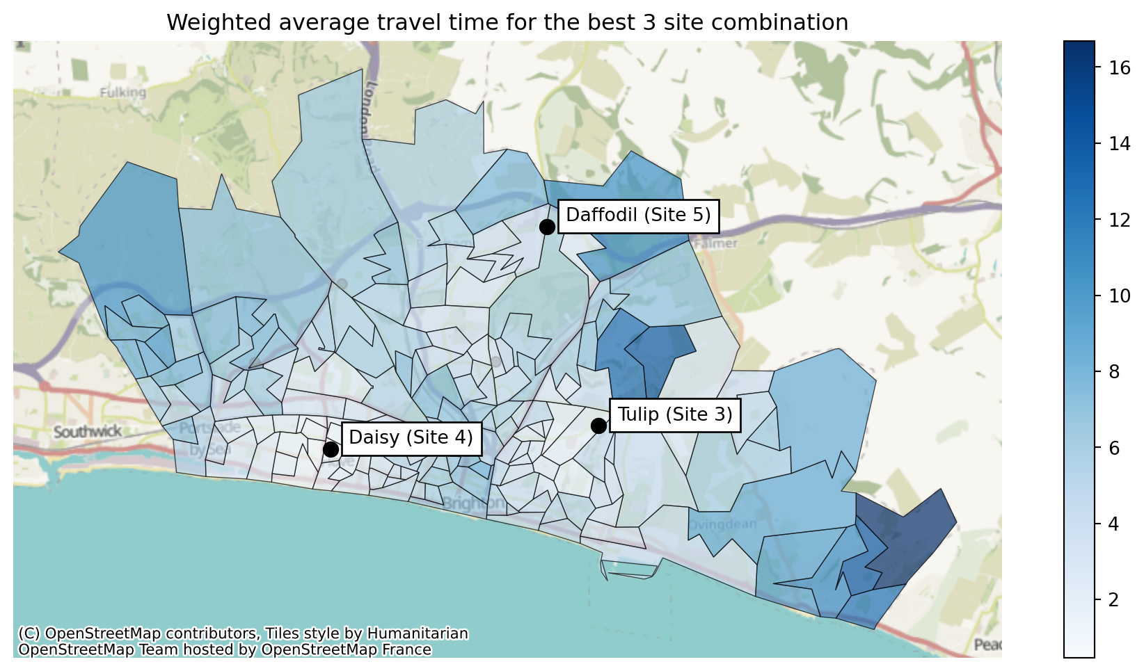

We could instead plot which site is the nearest to each location.

solutions.plot_best_combination(title="Site Allocation for the best 3 site combination", plot_site_allocation=True)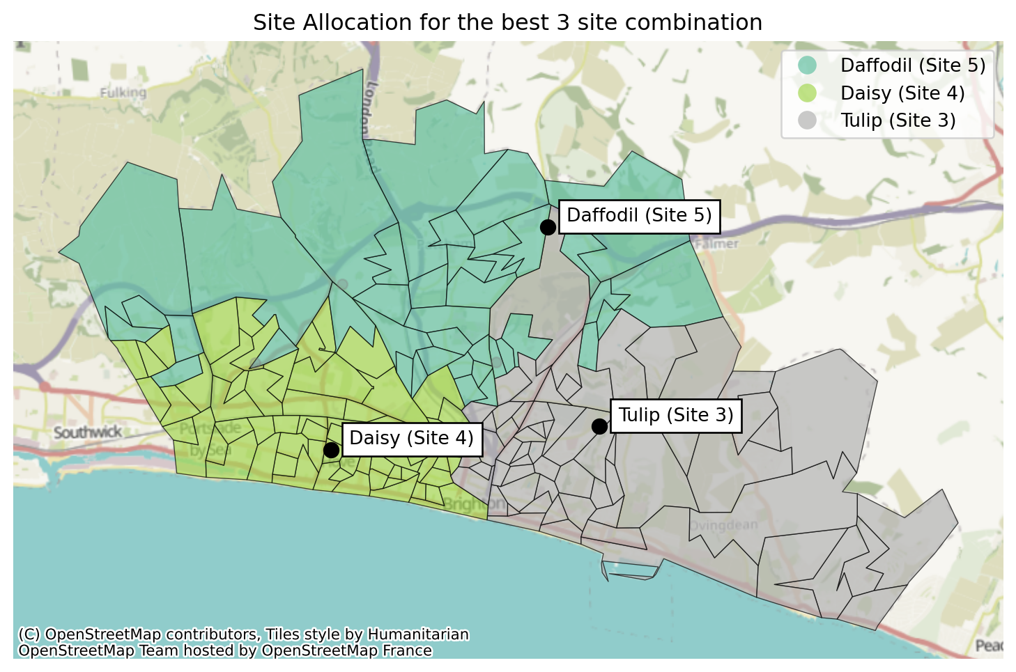

We can also choose to plot multiple possible combinations.

solutions.plot_n_best_combinations(subplot_title="Weighted Average car travel time:\n{solution['weighted_average'].values[0]:.2f} minutes")

(<Figure size 2880x1152 with 11 Axes>,
 array([<Axes: title={'center': 'Weighted Average car travel time:\n5.37 minutes'}>,
        <Axes: title={'center': 'Weighted Average car travel time:\n5.38 minutes'}>,
        <Axes: title={'center': 'Weighted Average car travel time:\n5.53 minutes'}>,
        <Axes: title={'center': 'Weighted Average car travel time:\n5.54 minutes'}>,
        <Axes: title={'center': 'Weighted Average car travel time:\n6.32 minutes'}>,
        <Axes: title={'center': 'Weighted Average car travel time:\n6.35 minutes'}>,
        <Axes: title={'center': 'Weighted Average car travel time:\n6.42 minutes'}>,
        <Axes: title={'center': 'Weighted Average car travel time:\n6.47 minutes'}>,
        <Axes: title={'center': 'Weighted Average car travel time:\n6.51 minutes'}>,
        <Axes: title={'center': 'Weighted Average car travel time:\n6.92 minutes'}>],
       dtype=object))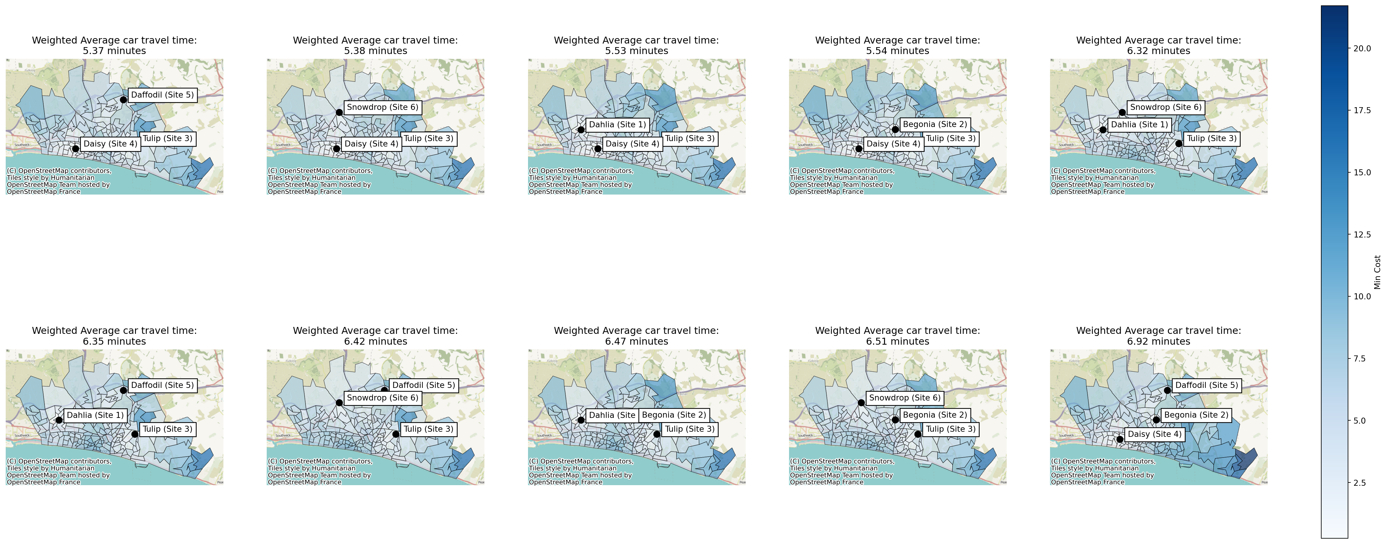

And like with the single solution plot, we can also switch to looking at the breakdown by the selected sites.

solutions.plot_n_best_combinations(plot_site_allocation=True, subplot_title="Weighted Average car travel time:\n{solution['weighted_average'].values[0]:.2f} minutes")

(<Figure size 2880x1152 with 10 Axes>,
 array([<Axes: title={'center': 'Weighted Average car travel time:\n5.37 minutes'}>,
        <Axes: title={'center': 'Weighted Average car travel time:\n5.38 minutes'}>,
        <Axes: title={'center': 'Weighted Average car travel time:\n5.53 minutes'}>,
        <Axes: title={'center': 'Weighted Average car travel time:\n5.54 minutes'}>,
        <Axes: title={'center': 'Weighted Average car travel time:\n6.32 minutes'}>,
        <Axes: title={'center': 'Weighted Average car travel time:\n6.35 minutes'}>,
        <Axes: title={'center': 'Weighted Average car travel time:\n6.42 minutes'}>,
        <Axes: title={'center': 'Weighted Average car travel time:\n6.47 minutes'}>,
        <Axes: title={'center': 'Weighted Average car travel time:\n6.51 minutes'}>,
        <Axes: title={'center': 'Weighted Average car travel time:\n6.92 minutes'}>],
       dtype=object))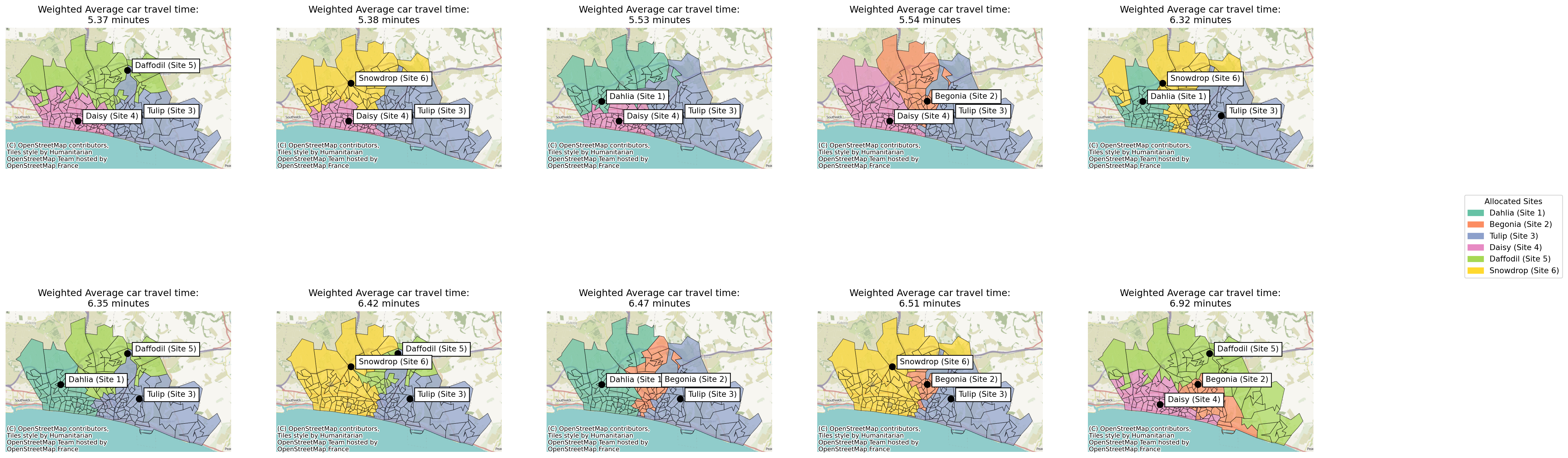

We can change what the solutions are ranked on - here we rate by the maximum travel time seen by any one LSOA, and display that instead.

solutions.plot_n_best_combinations(rank_on="max", subplot_title="Maximum car travel time:\n{solution['max'].values[0]:.2f} minutes")

(<Figure size 2880x1152 with 11 Axes>,
 array([<Axes: title={'center': 'Maximum car travel time:\n16.69 minutes'}>,
        <Axes: title={'center': 'Maximum car travel time:\n16.69 minutes'}>,
        <Axes: title={'center': 'Maximum car travel time:\n16.69 minutes'}>,
        <Axes: title={'center': 'Maximum car travel time:\n16.69 minutes'}>,
        <Axes: title={'center': 'Maximum car travel time:\n16.69 minutes'}>,
        <Axes: title={'center': 'Maximum car travel time:\n16.69 minutes'}>,
        <Axes: title={'center': 'Maximum car travel time:\n16.69 minutes'}>,
        <Axes: title={'center': 'Maximum car travel time:\n16.69 minutes'}>,
        <Axes: title={'center': 'Maximum car travel time:\n16.69 minutes'}>,
        <Axes: title={'center': 'Maximum car travel time:\n16.69 minutes'}>],
       dtype=object))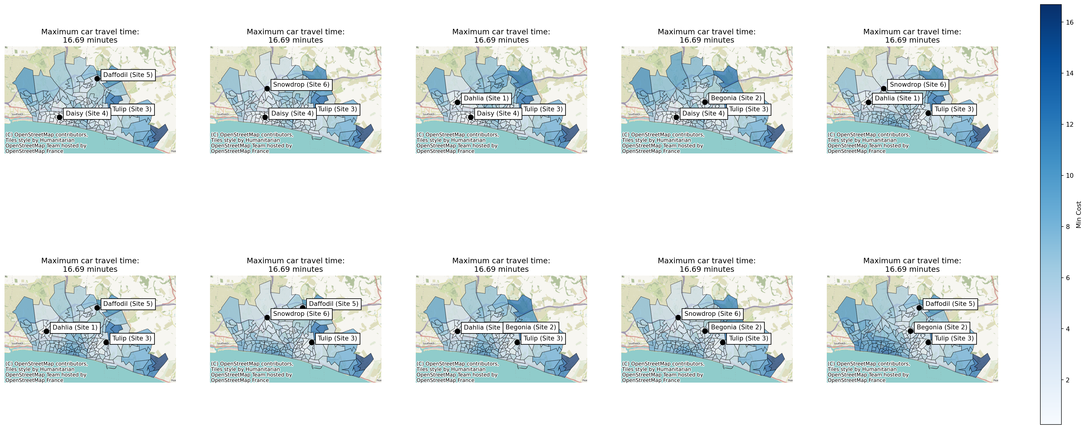

Plotting solution comparisons

solutions.plot_n_best_combinations_bar(n_best=10, interactive=True)

solutions.plot_n_best_combinations_bar(n_best=10, interactive=False)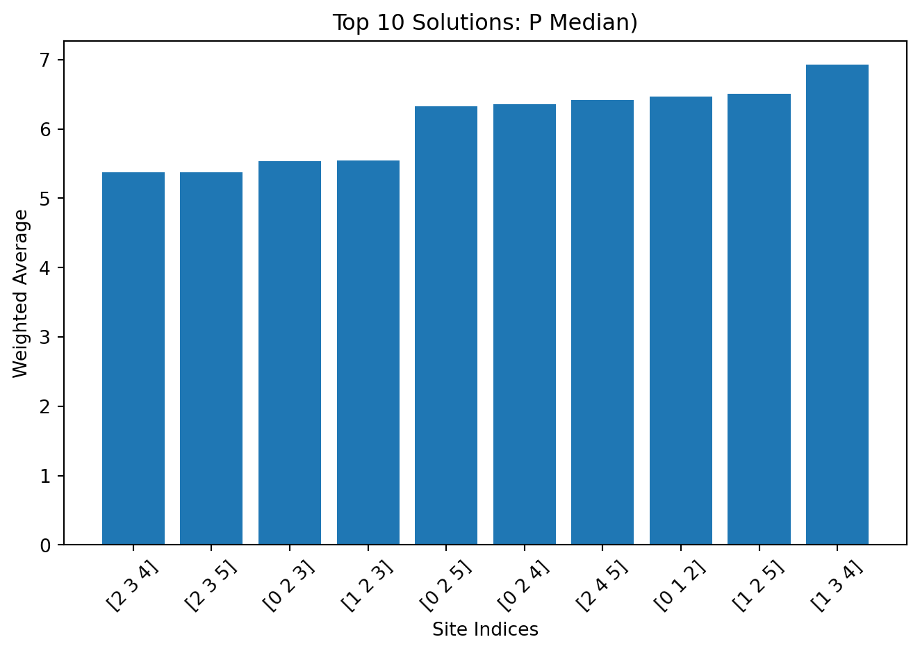

Let’s also look at how this varies when we compare the

solutions.plot_simple_pareto_front()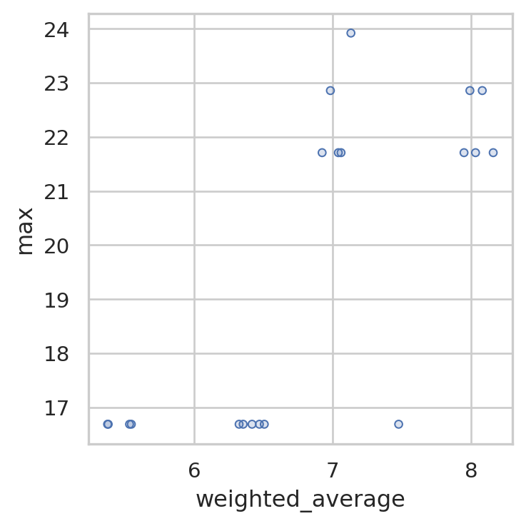

solutions.show_solutions()

	site_names	site_indices	coverage_threshold	weighted_average	unweighted_average	90th_percentile	max	problem_df
0	None	[2, 3, 4]	None	5.37	5.45	8.50	16.69	LSOA L...
1	None	[2, 3, 5]	None	5.38	5.36	8.06	16.69	LSOA L...
2	None	[0, 2, 3]	None	5.53	5.67	9.36	16.69	LSOA L...
3	None	[1, 2, 3]	None	5.54	5.59	9.00	16.69	LSOA L...
4	None	[0, 2, 5]	None	6.32	6.21	9.33	16.69	LSOA L...
5	None	[0, 2, 4]	None	6.35	6.32	9.70	16.69	LSOA L...
6	None	[2, 4, 5]	None	6.42	6.29	9.26	16.69	LSOA L...
7	None	[0, 1, 2]	None	6.47	6.39	9.77	16.69	LSOA L...
8	None	[1, 2, 5]	None	6.51	6.31	9.45	16.69	LSOA L...
9	None	[1, 3, 4]	None	6.92	6.76	11.32	21.71	LSOA L...
10	None	[1, 3, 5]	None	6.98	6.64	11.58	22.86	LSOA L...
11	None	[0, 3, 4]	None	7.04	6.81	12.26	21.71	LSOA L...
12	None	[3, 4, 5]	None	7.06	6.73	12.26	21.71	LSOA L...
13	None	[0, 1, 3]	None	7.13	6.92	11.93	23.92	LSOA L...
14	None	[1, 2, 4]	None	7.48	7.46	11.57	16.69	LSOA L...
15	None	[0, 1, 4]	None	7.95	7.66	11.67	21.71	LSOA L...
16	None	[0, 1, 5]	None	7.99	7.54	11.90	22.86	LSOA L...
17	None	[1, 4, 5]	None	8.03	7.65	11.67	21.71	LSOA L...
18	None	[0, 3, 5]	None	8.08	7.69	13.72	22.86	LSOA L...
19	None	[0, 4, 5]	None	8.16	7.70	12.65	21.71	LSOA L...

solutions.plot_all_metric_pareto_front()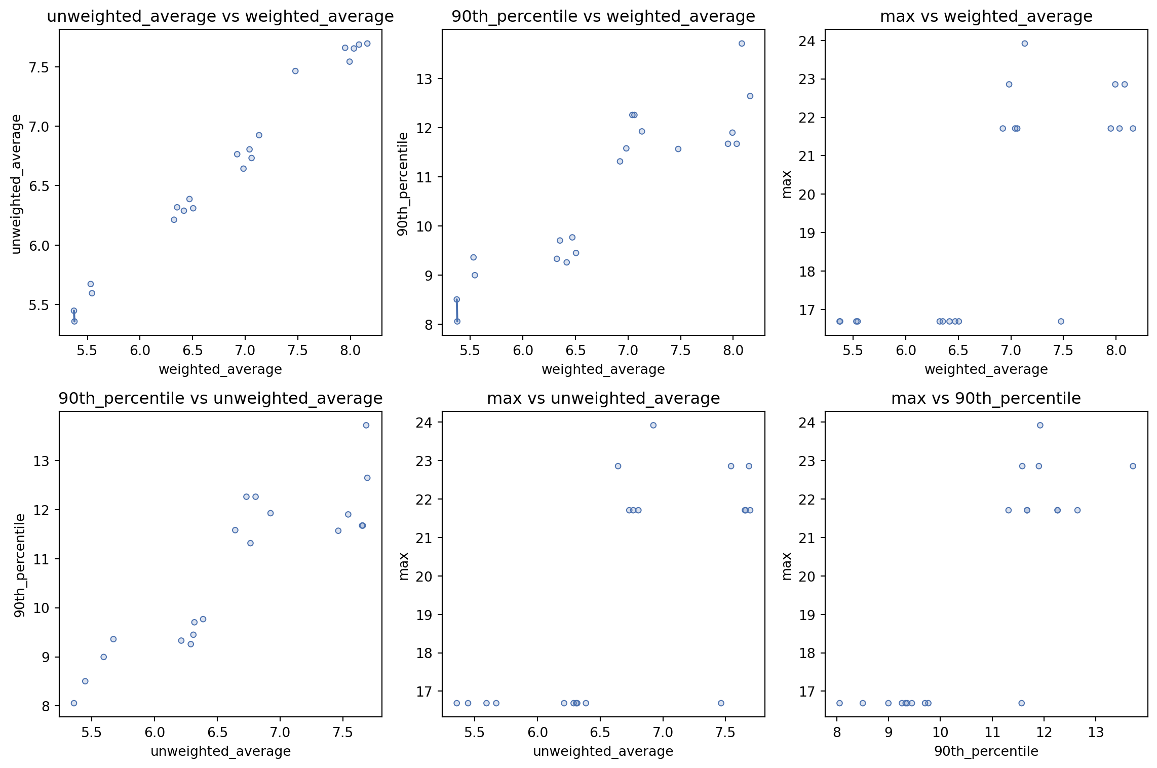

Try all different possible combinations

Let’s now explore the variation we see with a range of sites.

solutions_5 = problem.solve(p=5, objectives="p_median")
solutions_5.show_solutions()

	site_names	site_indices	coverage_threshold	weighted_average	unweighted_average	90th_percentile	max	problem_df
0	None	[0, 2, 3, 4, 5]	None	4.96	4.88	7.42	16.69	LSOA L...
1	None	[0, 1, 2, 3, 4]	None	4.99	5.00	7.78	16.69	LSOA L...
2	None	[1, 2, 3, 4, 5]	None	5.02	4.93	7.42	16.69	LSOA L...
3	None	[0, 1, 2, 3, 5]	None	5.05	4.90	7.67	16.69	LSOA L...
4	None	[0, 1, 2, 4, 5]	None	5.97	5.79	9.07	16.69	LSOA L...
5	None	[0, 1, 3, 4, 5]	None	6.51	6.20	11.32	21.71	LSOA L...

solutions_4 = problem.solve(p=4, objectives="p_median")
solutions_4.show_solutions()

	site_names	site_indices	coverage_threshold	weighted_average	unweighted_average	90th_percentile	max	problem_df
0	None	[0, 2, 3, 4]	None	5.08	5.12	7.82	16.69	LSOA L...
1	None	[2, 3, 4, 5]	None	5.11	5.05	7.42	16.69	LSOA L...
2	None	[1, 2, 3, 5]	None	5.20	5.07	7.75	16.69	LSOA L...
3	None	[0, 1, 2, 3]	None	5.22	5.21	8.34	16.69	LSOA L...
4	None	[0, 2, 3, 5]	None	5.23	5.19	8.06	16.69	LSOA L...
5	None	[1, 2, 3, 4]	None	5.28	5.33	8.32	16.69	LSOA L...
6	None	[0, 2, 4, 5]	None	6.05	5.90	9.07	16.69	LSOA L...
7	None	[0, 1, 2, 5]	None	6.14	5.92	9.33	16.69	LSOA L...
8	None	[0, 1, 2, 4]	None	6.24	6.17	9.69	16.69	LSOA L...
9	None	[1, 2, 4, 5]	None	6.33	6.17	9.26	16.69	LSOA L...
10	None	[0, 1, 3, 4]	None	6.63	6.43	11.32	21.71	LSOA L...
11	None	[1, 3, 4, 5]	None	6.66	6.37	11.32	21.71	LSOA L...
12	None	[0, 1, 3, 5]	None	6.83	6.48	11.58	22.86	LSOA L...
13	None	[0, 3, 4, 5]	None	6.91	6.56	12.26	21.71	LSOA L...
14	None	[0, 1, 4, 5]	None	7.67	7.27	11.67	21.71	LSOA L...

solutions_3 = problem.solve(p=3, objectives="p_median")
solutions_3.show_solutions()

	site_names	site_indices	coverage_threshold	weighted_average	unweighted_average	90th_percentile	max	problem_df
0	None	[2, 3, 4]	None	5.37	5.45	8.50	16.69	LSOA L...
1	None	[2, 3, 5]	None	5.38	5.36	8.06	16.69	LSOA L...
2	None	[0, 2, 3]	None	5.53	5.67	9.36	16.69	LSOA L...
3	None	[1, 2, 3]	None	5.54	5.59	9.00	16.69	LSOA L...
4	None	[0, 2, 5]	None	6.32	6.21	9.33	16.69	LSOA L...
5	None	[0, 2, 4]	None	6.35	6.32	9.70	16.69	LSOA L...
6	None	[2, 4, 5]	None	6.42	6.29	9.26	16.69	LSOA L...
7	None	[0, 1, 2]	None	6.47	6.39	9.77	16.69	LSOA L...
8	None	[1, 2, 5]	None	6.51	6.31	9.45	16.69	LSOA L...
9	None	[1, 3, 4]	None	6.92	6.76	11.32	21.71	LSOA L...
10	None	[1, 3, 5]	None	6.98	6.64	11.58	22.86	LSOA L...
11	None	[0, 3, 4]	None	7.04	6.81	12.26	21.71	LSOA L...
12	None	[3, 4, 5]	None	7.06	6.73	12.26	21.71	LSOA L...
13	None	[0, 1, 3]	None	7.13	6.92	11.93	23.92	LSOA L...
14	None	[1, 2, 4]	None	7.48	7.46	11.57	16.69	LSOA L...
15	None	[0, 1, 4]	None	7.95	7.66	11.67	21.71	LSOA L...
16	None	[0, 1, 5]	None	7.99	7.54	11.90	22.86	LSOA L...
17	None	[1, 4, 5]	None	8.03	7.65	11.67	21.71	LSOA L...
18	None	[0, 3, 5]	None	8.08	7.69	13.72	22.86	LSOA L...
19	None	[0, 4, 5]	None	8.16	7.70	12.65	21.71	LSOA L...

solutions_2 = problem.solve(p=2, objectives="p_median")
solutions_2.show_solutions()

	site_names	site_indices	coverage_threshold	weighted_average	unweighted_average	90th_percentile	max	problem_df
0	None	[2, 3]	None	5.94	6.21	10.46	16.69	LSOA L...
1	None	[2, 5]	None	6.69	6.60	9.45	16.69	LSOA L...
2	None	[0, 2]	None	6.81	6.88	10.19	16.69	LSOA L...
3	None	[3, 4]	None	7.33	7.14	12.26	21.71	LSOA L...
4	None	[1, 3]	None	7.46	7.31	11.93	23.92	LSOA L...
5	None	[2, 4]	None	7.61	7.62	11.58	16.69	LSOA L...
6	None	[3, 5]	None	8.23	7.85	13.72	22.86	LSOA L...
7	None	[1, 5]	None	8.36	7.93	11.90	22.86	LSOA L...
8	None	[0, 1]	None	8.45	8.15	11.98	23.92	LSOA L...
9	None	[4, 5]	None	8.52	8.08	12.65	21.71	LSOA L...
10	None	[0, 4]	None	8.56	8.20	12.65	21.71	LSOA L...
11	None	[1, 2]	None	8.69	8.77	14.30	16.69	LSOA L...
12	None	[0, 3]	None	9.19	8.96	15.21	26.33	LSOA L...
13	None	[1, 4]	None	9.19	8.95	12.19	21.71	LSOA L...
14	None	[0, 5]	None	9.39	8.86	14.26	22.86	LSOA L...

solutions_1 = problem.solve(p=1, objectives="p_median")
solutions_1.show_solutions()

	site_names	site_indices	coverage_threshold	weighted_average	unweighted_average	90th_percentile	max	problem_df
0	None	[2]	None	9.74	10.17	16.72	19.57	LSOA L...
1	None	[5]	None	9.75	9.25	14.26	22.86	LSOA L...
2	None	[4]	None	9.89	9.56	13.24	21.71	LSOA L...
3	None	[3]	None	9.97	9.84	16.95	26.82	LSOA L...
4	None	[1]	None	10.67	10.54	15.01	23.92	LSOA L...
5	None	[0]	None	11.79	11.25	17.47	26.33	LSOA L...

Let’s combine these into a single dataframe with the best solution for each (ranked on the weighted average).

all_sols = pd.concat(
    [solutions_1.solution_df.head(1),
     solutions_2.solution_df.head(1),
     solutions_3.solution_df.head(1),
     solutions_4.solution_df.head(1),
     solutions_5.solution_df.head(1)]
)

all_sols

site_names	site_indices	coverage_threshold	weighted_average	unweighted_average	90th_percentile	max	problem_df
None	[2]	None	9.738592	10.167285	16.720433	19.571000	LSOA L...
None	[2, 3]	None	5.943984	6.207341	10.461133	16.688833	LSOA L...
None	[2, 3, 4]	None	5.372208	5.447841	8.503100	16.688833	LSOA L...
None	[0, 2, 3, 4]	None	5.080178	5.115660	7.820333	16.688833	LSOA L...
None	[0, 2, 3, 4, 5]	None	4.957668	4.880920	7.417933	16.688833	LSOA L...

Finally, let’s plot the impact of different numbers of sites.

import plotly.express as px

all_sols["n_sites"] = all_sols["site_indices"].apply(lambda x: len(x))

px.bar(all_sols, x="n_sites", y="weighted_average", title="Weighted average travel time by number of sites")

px.bar(all_sols, x="n_sites", y="max", title="Maximum travel time by number of sites")

px.bar(all_sols, x="n_sites", y="90th_percentile", title="90th percentile travel time by number of sites")