As well as demand, equity, and other custom datasets, lokigi lets you attach a fixed cost to each candidate site – for example, the capital cost of building a new facility, or its ongoing running cost.
Pass a cost_col to add_sites() to register it. The total cost of whichever sites end up selected is always calculated and reported in solutions_df as total_cost, regardless of whether you use it for anything else.
from lokigi.site import SiteProblemproblem = SiteProblem()problem.add_sites("../../../sample_data/devon_cdcs_with_costs.csv", candidate_id_col="Facility_Name", vertical_geometry_col="Latitude", horizontal_geometry_col="Longitude", required_sites_col="Existing", cost_col="Build_Cost_GBP_Thousands", )problem.add_region_geometry_layer("../../../sample_data/LSOA_Devon_2021_EW_BSC_V4.gpkg", common_col="LSOA21NM" )problem.add_travel_matrix( travel_matrix_df="../../../sample_data/travel_matrix_car_devon_cdcs.csv", source_col="from_id", unit="minutes", )problem.add_demand("../../../sample_data/demand_MF_50_84.csv", demand_col="Total", location_id_col="LSOA 2021 Name" )problem.add_equity_data("../../../sample_data/devon_imd_2025_2021_LSOAs.csv", equity_col="Index of Multiple Deprivation (IMD) Decile (where 1 is most deprived 10% of LSOA", common_col="LSOA name (2021)", label="IMD Decile (1 = most deprived)" )
Guessed CRS: EPSG:4326 (Values fall within longitude/latitude bounds)
A quick look at site costs
devon_cdcs_with_costs.csv is a copy of the devon_cdcs.csv sample data used elsewhere in these examples, with an extra Build_Cost_GBP_Thousands column added.
The four Existing sites (which required_sites_col forces into every solution) have a cost of 0 – they’re already open, so there’s no new build cost for including them. The fourteen candidate sites range from roughly £240k to £620k to build.
By default (or with weights={"demand": 1.0}), total_cost is still calculated for every candidate solution – but it has no influence on which one is ranked best. Only travel time (weighted by demand) matters here.
The best solution adds Barnstaple - Archwood Retail Park to the four existing sites – purely because it gives the best average travel time. At £510k, it’s one of the more expensive candidates, but cost had no say in the decision.
Weighting by cost
Passing "cost" in the weights dictionary tells lokigi to take total_cost into account when comparing candidate solutions, alongside demand (and equity, if configured). It’s blended in using the same combination-level, batch-relative comparison used to rank solutions across every search strategy (brute-force, greedy, and grasp).
Note
weights={"cost": ...} requires cost_col to have been passed to add_sites() first – otherwise lokigi raises a clear KeyError telling you to add site costs before weighting by them (see below).
Now Okehampton - Exeter Road Industrial Estate is selected instead – roughly half the build cost of Barnstaple (£260k vs £510k), for a weighted average travel time barely 1% worse (20.43 vs 20.23 minutes). A strong trade in most planning contexts.
Exploring the cost/travel-time trade-off
Sweeping the balance between demand and cost shows how the chosen site shifts as cost is given more weight.
import pandas as pdsweep_rows = []for cost_weight in [0.0, 0.2, 0.4, 0.5, 0.6, 0.8, 1.0]: result = problem.solve( p=5, objectives="p_median", threshold_for_coverage=30, show_progress=False, weights={"demand": 1.0- cost_weight, "cost": cost_weight}, ) best = result.show_solutions().iloc[0] new_site = [ site for site in best["site_names"]if site notin problem.candidate_sites.loc[ problem.candidate_sites["Existing"] =="Yes", "Facility_Name" ].tolist() ] sweep_rows.append({"cost_weight": cost_weight,"new_site": new_site[0],"weighted_average": best["weighted_average"],"total_cost": best["total_cost"], })pd.DataFrame(sweep_rows)
cost_weight
new_site
weighted_average
total_cost
0
0.0
Barnstaple - Archwood Retail Park
20.23
510
1
0.2
Barnstaple - Archwood Retail Park
20.23
510
2
0.4
Okehampton - Exeter Road Industrial Estate
20.43
260
3
0.5
Okehampton - Exeter Road Industrial Estate
20.43
260
4
0.6
Okehampton - Exeter Road Industrial Estate
20.43
260
5
0.8
Okehampton - Exeter Road Industrial Estate
20.43
260
6
1.0
Holsworthy - Underlane
20.94
240
Three distinct tiers emerge as the cost weight increases, each cheaper than the last at the expense of a little travel time:
Cost only (1.0): Holsworthy - Underlane (£240k, 20.94 min)
Note
As with other weights, mixing objectives this way can be opaque and have limited effect on the outcome – as seen above, several weight combinations here produce identical results. For a more transparent way to explore cost/travel-time trade-offs, consider comparing solutions directly or a pareto-front approach treating cost as a second objective.
Combining cost with other weights
Cost composes with the rest of the weighting system just like any other key – here it’s blended alongside demand and equity in a single solve.
cost_col is entirely optional. If it’s never passed to add_sites(), everything works exactly as before: total_cost is reported as NaN in solutions_df, and attempting to weight by "cost" raises a clear error rather than silently doing nothing.
KeyError: "The following weight keys are missing from the problem data: ['cost']"
Comparing cost via a pareto front
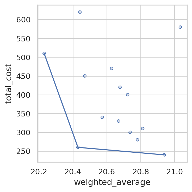
Rather than picking a single cost weight, we can treat total_cost as just another metric in a pareto front, exactly as in Multiobjective Optimisation with Pareto Fronts. This avoids having to choose an arbitrary weight, and instead surfaces every non-dominated cost/travel-time trade-off at once.
We’ll reuse solution_unweighted from earlier – total_cost was already calculated for every candidate solution regardless of weighting, so no re-solving is needed.
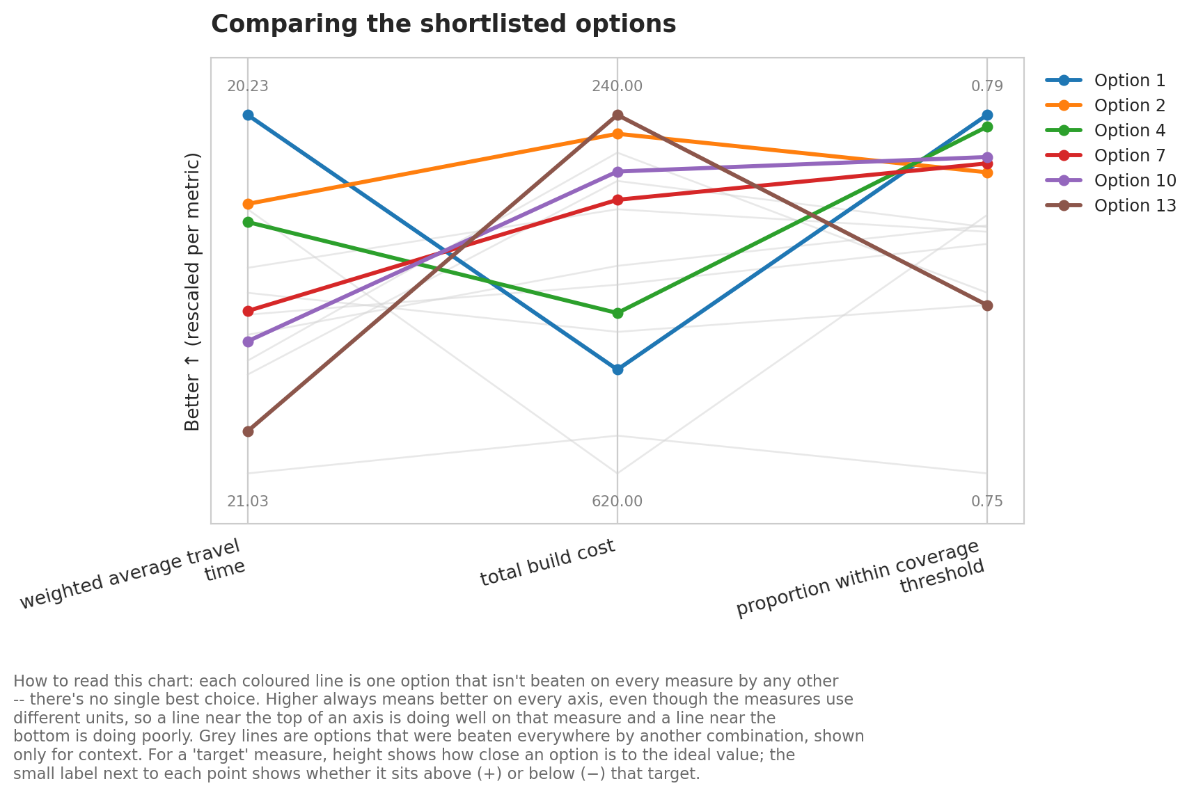
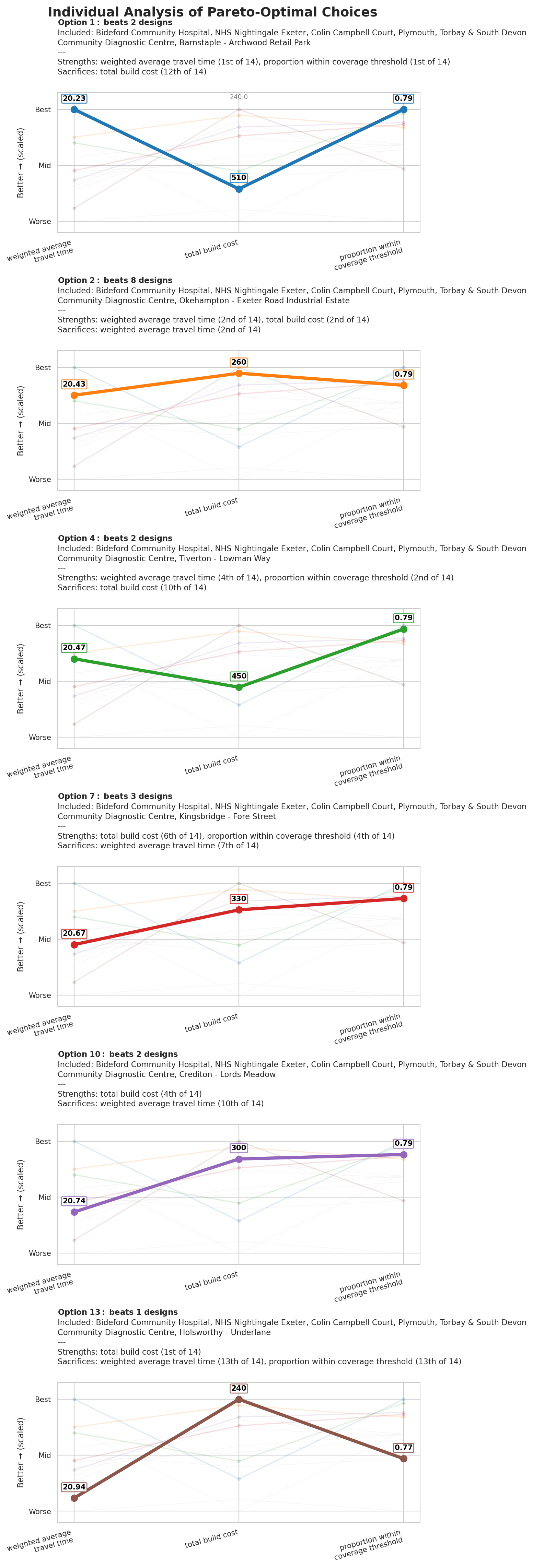
Bringing coverage into the picture grows the non-dominated set from three solutions to six – some of the cheaper options that were dominated on cost/travel-time alone turn out to offer better coverage than their neighbours, so they earn a place back on the front.
pareto_summary() returns just these non-dominated solutions, sorted by the first metric in the list.
solution_unweighted.pareto_summary()
solution_rank
weighted_average
total_cost
proportion_within_coverage_threshold
0
1
20.230707
510
0.791487
1
2
20.429983
260
0.785538
2
4
20.470531
450
0.790269
3
7
20.669638
330
0.786461
4
10
20.737475
300
0.787119
5
13
20.938731
240
0.771772
We can also visualise every non-dominated solution across all three metrics at once with plot_pareto_summary() – as before, values further up each axis are always better, cost included.